Greenhouse Design And Control By Pedro Ponce 2i6d33
This document was ed by and they confirmed that they have the permission to share it. If you are author or own the copyright of this book, please report to us by using this report form. Report 445h4w
Overview 1s532p
& View Greenhouse Design And Control By Pedro Ponce as PDF for free.
More details 6h715l
- Words: 102,552
- Pages: 378
Ponce, Molina, Cepeda, Lugo & MacCleery
an informa business
Greenhouse Design and Control
Agricultural production is one of the main keys to the development of healthy societies. It is anticipated that agricultural systems will increasingly have to contend with temperature, humidity and water stress in the near future. This makes the need to increase the efficiency of land and water use ever more urgent. The control and design of greenhouses allows to increase dramatically the quality of crops and extend the cultivation period year-round. A properly designed autonomous greenhouse based on hydroponics can greatly reduce the amounts of nutrients and energy expended in agricultural production. This book deals with different types of greenhouses, materials, structures, advanced control techniques and tendencies that are needed for deg and controlling an advanced greenhouse. The control system is presented as an integral system which covers the explanation of basic and advanced concepts for a real time controller. Also, structural analysis is introduced, whereby mechanical design is regarded as a key factor. The book incorporates simulations and experimental results, and utilizes LabVIEW and ADAMS software. Finally, it provides a perspective on the present state and future of greenhouses globally. Written in a highly accessible manner, this book will prove useful to horticulturalists, agricultural engineers, greenhouse engineers and designers. Its easy-to-absorb contents are also suitable for (under)graduate students and researchers in agricultural and electronic engineering, horticulture, crop cultivation and soft computing.
Greenhouse Design and Control Pedro Ponce Arturo Molina Paul Cepeda Esther Lugo Brian MacCleery
Greenhouse Design and Control
This page intentionally left blank
Greenhouse Design and Control
Pedro Ponce, Arturo Molina, Paul Cepeda & Esther Lugo Tecnologico de Monterrey, Campus Ciudad de Mexico, Mexico City, Mexico
Brian MacCleery National Instruments, Austin,TX, USA
CRC Press/Balkema is an imprint of the Taylor & Francis Group, an informa business © 2015 Taylor & Francis Group, London, UK Typeset by MPS Limited, Chennai, India Printed and Bound by I Group (UK) Ltd, Croydon, CR0 4YY All rights reserved. No part of this publication or the information contained herein may be reproduced, stored in a retrieval system, or transmitted in any form or by any means, electronic, mechanical, by photocopying, recording or otherwise, without written prior permission from the publisher. Although all care is taken to ensure integrity and the quality of this publication and the information herein, no responsibility is assumed by the publishers nor the author for any damage to the property or persons as a result of operation or use of this publication and/or the information contained herein. Library of Congress Catag-in-Publication Data Ponce Cruz, Pedro. Greenhouse design and control / authors, Pedro Ponce,Arturo Molina, Paul Cepeda & Esther Lugo, InstitutoTecnologico de Monterrey, Ejidos de Huipulco, Mexico, Brian MacCleery, National Instruments,Austin,TX, USA. — First edition. pages cm Includes bibliographical references and index. ISBN 978-1-138-02629-2 (hardback) — ISBN 978-1-315-77155-7 (ebook) 1. Greenhouses–Design and construction. I. Title. SB416.P66 2014 635.9’823—dc23 2014016067 Published by: CRC Press/Balkema P.O. Box 11320, 2301 EH Leiden,The Netherlands e-mail: [email protected] www.crress.com – www.taylorandfrancis.com ISBN: 978-1-138-02629-2 (Hbk) ISBN: 978-1-315-77155-7 (eBook)
Pedro To my charming and lovely Norma who is my inspiration every single day of my life. Arturo To my wife Silvia and lovely kids Julio and Monse. In memory of my mom Rosita. Paul I dedicate this work to my father in heaven and my beautiful family: Francisco,Ana María, María José, Rosa, Ruby, David, Carlos, Nathan, whose , patience and love are the search engine for a better future. Selvia, you’re part of this, thank you for living through and sharing hours of work, effort and dedication, encouraging me in difficult times and celebrating the best of times. To my colleagues and co-authors, thank you for the opportunities provided. Finally, this is also for all the people not mentioned here and who have been part of my growth and achievements. Esther To the ITESM CCM for all the for this research that has become part of this book. To my tutor Dr. Pedro Ponce for the opportunity to participate in this research work. To my parents, brothers, sister and cousin, for ing me. To my boyfriend for the , time and ideas for improving this research. To my friends for the time and help they have given me to perform my job. Brian To Eva Jane MacCleery, greenhouse for my spirit.
This page intentionally left blank
Table of contents
List of figures List of tables Preface How to read this book
xi xix xxiii xxv
1
Introduction 1.1 Greenhouse motivation 1.1.1 The state of North American protected agriculture
1 11 20
2
State of the art: greenhouse and controls
29
3
Greenhouse fundamentals 3.1 Greenhouse generalities and construction 3.1.1 Site selection 3.1.2 Orientation 3.1.3 Plan layout 3.1.4 Availability of water 3.1.5 Availability of electricity 3.1.6 Structure design 3.1.7 Standards for the construction 3.1.8 Greenhouse costs
41 43 44 45 46 48 48 51 59 64
4
Greenhouse materials and structures 4.1 Structural materials 4.1.1 Structural conformation 4.2 Cladding materials 4.3 Foundations and floor materials 4.3.1 Connections and clamps 4.3.2 Leaks 4.3.3 Windbreak 4.3.4 Insect screens 4.4 Eco-materials 4.5 Material selection for a greenhouse 4.6 Material properties of a tunnel type greenhouse 4.6.1 Tunnel fixed Zenith ventilation greenhouses 4.6.2 Simulation in the Inventor® program
67 71 73 74 79 80 81 81 81 82 83 85 85 88
viii Table of contents
4.7
4.8 5
6
4.6.3 Characteristics of the loads that are applied to the structure 4.6.4 CFD simulator by Inventor® Greenhouse construction standards 4.7.1 Materials used in the structures 4.7.2 Norms of materials 4.7.3 Activities for greenhouse construction Structures and environmental control
93 107 115 115 116 117 119
Greenhouse automation and control 5.1 Real time control system and greenhouses 5.2 Advanced control systems for portable greenhouses 5.2.1 Basic portable greenhouse description 5.2.2 Advanced control systems 5.3 Control implementation 5.3.1 Portable greenhouse results 5.4 Constituents of controlled environment for conventional greenhouses 5.5 Sensors for greenhouse monitoring 5.6 Automation systems 5.7 Advanced protected systems – hydroponics 5.7.1 Nutrient film technique 5.8 Greenhouse modeling and control 5.8.1 Greenhouse models 5.9 Types of controls 5.9.1 Control techniques theory 5.9.2 Bang-bang or on/off control 5.9.3 PID control 5.9.4 /feed-forward linearization 5.9.5 Sliding modes 5.9.5.1 Fuzzy logic control 5.9.6 Adaptive neural fuzzy inference system – ANFIS 5.9.7 Green tech control and supervisor
127 129 140 144 145 147 150 171 182 199 220 224 226 226 230 236 236 237 238 241 244 247 250
Basic greenhouse control design and implementation 6.1 Mechanical systems 6.1.1 Structure and materials selection 6.1.2 Ventilation systems 6.1.3 Shading system 6.1.4 Water fogging system 6.1.5 Irrigation system 6.1.6 Sensors 6.2 Electrical and electronic system 6.3 Control system for greenhouses 6.3.1 Intelligent control system development 6.3.2 LabVIEW™ controllers programming 6.3.3 Intelligent controllers simulation 6.3.4 Graphical interface (GUI) and functions
257 259 259 262 264 266 268 270 282 284 291 296 299 303
Table of contents ix
6.4
7
Control results 6.4.1 Intelligent controllers simulation results 6.4.2 PID-type controller simulation results 6.4.3 On/off controllers experimental results 6.4.4 Intelligent controllers experimental results 6.4.5 Analysis of control systems
Automatic greenhouse operation 7.1 Field versus greenhouse grown fruit 7.2 Plant forms 7.3 Photosynthetic characteristics 7.4 Temperature requirements 7.5 Carbon dioxide 7.6 Light quality and intensity 7.7 Water requirement 7.8 Factors affecting greenhouse production 7.9 Greenhouse structures 7.10 Pest management 7.11 Culture systems 7.12 Plant nutrition 7.13 General greenhouse reference conditions
References Subject index
306 308 315 319 324 328 331 332 333 333 334 335 334 335 336 337 338 338 339 341 343 351
This page intentionally left blank
List of figures
1.1 1.2 1.3 1.4 1.5 1.6 1.7 1.8 1.9 1.10 1.11 1.12 1.13 1.14 1.15 1.16 1.17 1.18 1.19 1.20 1.21 1.22 1.23 1.24 2.1 2.2 2.3 3.1 3.2 3.3 3.4 3.5 3.6 3.7 3.8
Micro-tunnels Macro-tunnel Shade House Greenhouses Almería, Spain Total Area in Major Greenhouse Production Countries Protected Crops in the World: over 3 million hectares Countries using Hydroponics FAO Food Price Index Actual worldwide population involved in agriculture World’s Population Dynamics Undernourishment in 2011–2013, by Region Temperature Rise Predictions Impact of Climate Change in the 2080s on Agricultural Productivity The Temperature Effect on Photosynthesis and Respiration Composition of Agricultural Area by Region Traditional Over Protected Agriculture North American Greenhouse Production Distribution Actual Mexican Population Composition of Agricultural Area in Mexico Mexico: Main Macroeconomic Indicators, 1995–2011 Panorama of Protected Agriculture in Mexico Greenhouse Sector Development in Mexico Protected Agriculture Crops in Mexico Dutch Style Greenhouse The Orangerie at Versailles English Greenhouse Classification of Greenhouse Systems Classification of Greenhouses based on Working Principles Location Priorities for Greenhouses based on Ambient Sunlight Plan Layout of a Greenhouse Along with other Facilities Benches and Beds Arrangements Greenhouse Solar System Wind Farm Greenhouse forms still in Use
2 2 3 4 5 6 7 8 12 13 13 14 15 16 17 18 20 21 23 23 24 25 25 26 29 30 30 42 43 46 47 47 50 50 51
xii
List of figures
3.9 3.10 3.11 3.12 3.13 3.14 3.15 3.16 4.1 4.2 4.3 4.4 4.5 4.6 4.7 4.8 4.9 4.10 4.11 4.12 4.13 4.14 4.15 4.16 4.17 4.18 4.19 4.20 4.21 4.22 4.23 4.24 4.25 4.26 4.27 4.28 4.29 4.30 4.31 4.32 4.33 4.34 4.35 4.36 4.37
Basic Structures of Greenhouse Ridge and Furrow Configuration of Greenhouse Structures Greenhouse Structure Designs based on Mexican Standard Arch Roof Greenhouse (Multi-Span) Saw Tooth Design Venlo House World Agro-Climatic Zones Design Loads on Different Greenhouse Structures Tunnel Fixed Zenith Greenhouses The Home Screen of Inventor® Selecting screen of work, learn or extend, Inventor® Configuration of the template, Inventor® First screen of the sketch in Inventor® Example of the auxiliary tools, Inventor® Sketch with general characteristics of the structure 3D sketch Approach characteristics of the structures Starting the structural analysis Displacement in the nodes of the greenhouses in mm Normal stresses in the greenhouse, MPa Moment of force MX in N mm Moment of force My in N mm Moment of force Mz in N mm Tension cut off Tx in Mpa Tension cut off Ty in Mpa Forces in Fx in N Forces in Fy in N Forces in Fz in N Torsional stresses in Mpa Dimensions of the greenhouse inside a Winter Tunnel Selection of the materials and the wind flow Boundary conditions in greenhouses Creation of elements in the structure of the greenhouses Post processing of the information with respect to the force applied in the greenhouses Wind analysis for a Tunnel Fixed Zenith greenhouse Wind analysis for a Butterfly greenhouse Wind analyses for a Sawtooth greenhouse Wind analysis for a Multi Tunnel greenhouse Wind analysis for a Modular Parral greenhouse Wind analysis for a Tunnel greenhouse Wind analysis for a Chapel greenhouse Wind analysis for a Chinese hat greenhouse Exchanges of fluxes in the greenhouse environment Activities for greenhouse construction Environmental controls inside greenhouses
52 53 53 54 56 57 58 63 86 88 89 90 90 91 92 93 93 94 98 98 99 99 100 100 101 101 102 102 103 109 109 110 110 111 111 112 112 113 113 114 114 114 116 119 122
List of figures xiii
5.1 5.2 5.3 5.4 5.5 5.6 5.7 5.8 5.9 5.10 5.11 5.12 5.13 5.14 5.15 5.16 5.17 5.18 5.19 5.20 5.21 5.22 5.23 5.24 5.25 5.26 5.27 5.28 5.29 5.30 5.31 5.32 5.33 5.34 5.35
Diagram of a Typical Hi-Tech Greenhouse Greenhouse Control Design Yields of Tomato Production in Greenhouse Technology Embedded System Architecture FPGA configurable logic and I/O blocks LabVIEW FPGA compiler NI cRIO-9024 Real-Time Controller and PID code for FPGA Reconfigurable FPGA Chassis There are more than 50 NI C Series I/O modules for CompactRIO to connect to almost any sensor or actuator (1 Host to 1 Target) Configuration A 1:N (1 host to N targets) configuration is common for systems controlled by a local operator Distributed Machine Control System LabVIEW FPGA Control on CompactRIO Sample Project Architecture LabVIEW Supervisory Control and Data Acquisition Sample Project Architecture Data Communication Diagram Sample Projects by CompactRIO Shows the fuzzy logic controller for a greenhouse that is an example of LabVIEW program Portable Greenhouse concept and experimental one using solar and wind energy Block diagram of a fuzzy control system Neuron model in artificial neural networks and LabVIEW perceptron program Dynamical neural network structure and LabVIEW Artificial Neural Network program (ICTL) Representation of a fuzzy-PD control Duty cycle signal as output in the proposed intelligent controller Five bell hip functions for input signals and LabVIEW program Seven triangular hip functions for output signal Step response of the 5-bell MF’s of the fuzzy-PD controller Quadratic error plot for the step response of the 5-bell MF’s of the fuzzy-PD controller Five triangular hip functions for input signals Step response of the 5-triangular MF’s of the fuzzy-PD controller Quadratic error plot for the step response of the 5-triangular MF’s of the fuzzy-PD controller Seven bell hip functions for input signals Five triangular hip functions for output signal Step response of the 7-bell MF’s of the fuzzy-PD controller Quadratic error plot for the step response of the 7-bell MF’s of the fuzzy-PD controller Seven triangular hip functions for input signals
127 128 129 131 132 133 134 135 135 136 137 137 138 140 141 141 143 144 145 146 147 148 149 151 152 153 153 154 154 155 156 156 157 157 158
xiv List of figures
5.36 5.37 5.38 5.39 5.40 5.41 5.42 5.43 5.44 5.45 5.46 5.47 5.48 5.49 5.50 5.51 5.52 5.53 5.54 5.55 5.56 5.57 5.58 5.59 5.60 5.61 5.62 5.63 5.64 5.65 5.66 5.67 5.68
Step response of the 7-triangular MF’s of the fuzzy-PD controller Quadratic error plot for the step response of the 7-triangular MF’s of the fuzzy-PD controller Seven singleton hip functions for output signal Step response of the 7-triangular input MF’s and 7-singleton output MF’s of the fuzzy-PD controller Quadratic error plot for the step response of the 7-triangular input MF’s and 7-singleton output MF’s of the fuzzy-PD controller Comparison between the five fuzzy-PD configurations for the light intensity controller Seven triangular hip functions for input signals Triangular hip functions for output signals Ramp response of the 5-bell MF’s fuzzy-PD temperature controller Quadratic error plot for the ramp response of the 5-bell fuzzy-PD temperature controller Five triangular hip functions for input signals Ramp response of the 5-triangular MF’s fuzzy-PD temperature controller Quadratic error plot for the ramp response of the 5-triangular fuzzy-PD temperature controller Seven bell hip functions for input signals Ramp response of the 7-bell MF’s fuzzy-PD temperature controller Quadratic error plot for the ramp response of the 7-bell fuzzy-PD temperature controller Seven triangular hip functions for input signals Ramp response of the 7-triangular MF’s fuzzy-PD temperature controller Quadratic error plot for the ramp response of the 7-triangular fuzzyPD temperature controller Comparison between the four fuzzy-PD configurations for the temperature controller Temperature neural network model plant Response of the temperature controller Quadratic error plot for the ramp response of the temperature neural network controller Light intensity neural network model plant Response of the light intensity controller Quadratic error plot for the step response of the light intensity neural network controller Response of the relative humidity on/off controller Energy Exchange between Greenhouse and Surroundings Effects of CO2 , Light and Temperature on Photosynthesis in Cucumber Solar Radiation for Different Greenhouse Designs and Orientations Types of Radiant Energy Rates of Photosynthetic Activity under Different Qualities of Light The Spectrum of Light Emissions of Lamps for Use in Greenhouses
158 158 159 159 159 160 160 161 162 162 163 164 164 164 165 165 166 166 167 167 168 168 168 169 169 170 170 172 173 176 176 177 178
List of figures xv
5.69 5.70 5.71 5.72 5.73 5.74 5.75 5.76 5.77 5.78 5.79 5.80 5.81 5.82 5.83 5.84 5.85 5.86 5.87 5.88 5.89 5.90 5.91 5.92 5.93 5.94 5.95 5.96 5.97 5.98 5.99 5.100 5.101 5.102 5.103 5.104 5.105 5.106 5.107 5.108 5.109 5.110 5.111 5.112 5.113 5.114 5.115
Relationship between CO2 , Light and Photosynthesis in Wheat Variation of CO2 Concentration in Greenhouse Different Soil-less Cultivation Methods Hydroponic Cultivation Method Sensor Phenomenon Use of Sensors in Greenhouses Sensor Signal Conditioning Some Op-Amp Configurations in Signal Conditioning Thermocouples Platinum Thin Film RTD Thermistors Capacitive Humidity Sensors Resistive Humidity Sensors Light Dependent Resistors Pyranometer Electrochemical CO2 Sensors Electrical Conductivity Probes pH Probes Cup Anemometer and Vane Rain Detector Electric Motor Derived Circuit Elements Variable Frequency Drive Components Electric and Physical Diagram of Basic Motor Elements Chimney Effect in General Ventilation Roll Up Side Greenhouse Ventilation Pad-and-Fan Cooling System and Water Trickling Arrangement Cooling Pad Fog Cooling Nozzle Convection-Tube Winter Cooling System Fan Arrangements for HAF System Unit Heater used with Convection-Tube Air Distribution System Arrangement of Heating Pipe Coils A Typical Solar Heating System Basic Theory: Heat Collection Heat Pump Schematic Schematic Diagram Perimeter Watering System Sprinkler Irrigation System Boom Watering Basic Components of a Trickle Irrigation System Tomato Production using Hydroponics NFT Hydroponic System Greenhouse Climate Dynamic Model Thermostat Dedicated Microprocessor for Controlling Greenhouse Environment Computerized Control Systems in Greenhouse On/Off Controller Behavior On/Off Controller whit Hysteresis Behavior
179 179 181 182 182 183 185 186 189 189 190 191 192 193 194 195 197 197 198 199 200 201 202 204 204 205 206 207 208 210 211 212 213 214 214 217 217 219 219 222 225 227 232 234 235 236 237
xvi
List of figures
5.116 5.117 5.118 5.119 5.120 5.121 5.122 5.123
PID Controller Response Trajectories in the Portrait Phase The Chattering Phenomenon Complete fuzzy Inference System Commonly used Fuzzy If-Then Rules and Fuzzy Mechanism ANFIS General Structure Greenhouse Control Loop Schematic Green Tech Control and Supervisor was Patented by Tecnologico de Monterrey Ciudad de Mexico (P. Ponce et al., 2012) 5.124 Case Analysis for Different Operating Points 5.125 PD Fuzzy Control Loop 5.126 Inputs hip Functions 6.1 Greenhouse Site Selection and Orientation 6.2 Block Diagram of the Whole Cultivation Field Control System 6.3 Intelligent Greenhouse Structure – CAD 6.4 Intelligent Greenhouse Structure + Cladding + Floor − CAD 6.5 Intelligent Greenhouse – First Stages of Construction 6.6 Vent System (Side-wall or Zenith) – CAD 6.7 Exhaust Fan – CAD 6.8 Natural Ventilation System 6.9 Exhaust Fan + Structure + Micro-tunnel 6.10 Shading System – CAD 6.11 Shade Meshes 6.12 Shading Mesh System 6.13 Water Fogging System (Humidifier) – CAD 6.14 Shading Mesh System 6.15 Hydroponics and Nutrient Supply System – CAD 6.16 PVC Pipe System 6.17 Hydroponic System Components 6.18 Nutrient Storage Tanks 6.19 Electro-valve System 6.20 ASCO Electro-valve 6.21 Intelligent Greenhouse – CAD 6.22 Intelligent Greenhouse Summary 6.23 Sensors Location 6.24 Temperature/Humidity Sensor – PH1 125 6.25 Temperature/Humidity Sensor Shield 6.26 Connection Mode of a LDR 6.27 LDR 6.28 pH and EC Probes 6.29 Electrical Conductivity Circuit 6.30 pH Circuit 6.31 Printed Circuits, Power Supply and Casing 6.32 PING))) Ultrasonic Sensor Principle 6.33 PING))) Ultrasonic Sensor 6.34 National Instruments Hardware – DAQ Systems 6.35 Electric/Electronic System Diagram
238 241 242 246 247 248 250 251 252 254 254 258 258 259 260 261 262 262 263 264 265 265 266 267 267 269 269 270 271 271 272 273 274 275 275 276 276 277 279 279 279 280 280 281 283 285
List of figures xvii
6.36 6.37 6.38 6.39 6.40 6.41 6.42 6.43 6.44 6.45 6.46 6.47 6.48 6.49 6.50 6.51 6.52 6.53 6.54 6.55 6.56 6.57 6.58 6.59 6.60 6.61 6.62 6.63 6.64 6.65 6.66 6.67 6.68 6.69 6.70 6.71 6.72 6.73 6.74 6.75 6.76 6.77 6.78 6.79 6.80 6.81 6.82
Electrical/Electronic System Electrical Cabinets and Control Computer Climatic Control Loop Nutrient Supply System Nutrient Supply Fuzzy Model Neural Network Configuration Input hip Functions Nutrient Supply Control Loop Generic On/Off Controller Flow Diagram Conventional On/Off Temperature Control Conventional On/Off Relative Humidity Control Conventional On/Off Light Intensity Control Conventional On/Off Electrical Conductivity Control Non-linear Temperature and Relative Humidity Control Sliding Modes + /Feed-forward Linearization Fuzzy Logic Electrical Conductivity Control Irrigation Timer Control Simulation Graphical Interface Simulation Block Diagram: Climate Control Simulation Block Diagram: Nutrient Supply Control Recorded Temperature and Relative Humidity – June 15/2012 Recorded Temperature and Relative Humidity – December 15/2012 Recorded Temperature and Relative Humidity – April 15/2013 GUI – Program Start GUI – Creating a New Crop I GUI – Open an Existing Crop II GUI – Program Summary GUI – Controller Choice GUI – Main Interface GUI – Manual Control Temperature Response Set Point Change Relative Humidity Response Set Point Change Ventilation Response Set Point Change Fogging System Response Set Point Change Temperature Response Disturbance Change Relative Humidity Response Disturbance Change Ventilation Response Disturbance Change Fogging System Response Disturbance Change Electrical Conductivity Response Set Point Change Valve Time Response Set Point Change Temperature Response Set Point Change Relative Humidity Response Set Point Change Ventilation Response Set Point Change Fogging System Response Set Point Change Temperature Response Disturbance Change Relative Humidity Response Disturbance Change Ventilation Response Disturbance Change
291 292 293 294 295 296 296 297 297 298 298 299 299 300 300 301 301 302 302 303 303 304 304 305 305 306 307 307 308 309 310 310 311 311 312 312 313 313 314 314 315 316 316 317 317 318 318
xviii
6.83 6.84 6.85 6.86 6.87 6.88 6.89 6.90 6.91 6.92 6.93 6.94 6.95 6.96 6.97 6.98
List of figures
Fogging System Response Disturbance Change Temperature Response On/Off Controller Ventilation Response On/Off Controller Relative Humidity Response On/Off Controller Fogging System Response On/Off Controller Light Intensity Response On/Off Controller Shadow Mesh Response On/Off Controller Electrical Conductivity Response On/Off Controller Electro-valve Response On/Off Controller Irrigation Pump Response Temperature Response Non-Linear Controller Relative Humidity Response Non-Linear Controller Ventilation Response Non-Linear Controller Fogging System Response Non-Linear Controller Electrical Conductivity Response Fuzzy Controller Electro-valve Response Fuzzy Controller
319 320 320 321 321 322 322 323 323 324 325 325 326 326 327 327
List of tables
1.1 1.2 1.3 1.4 1.5 1.6 1.7 1.8 1.9 3.1 3.2 3.3 3.4 3.5 3.6 3.7 3.8 3.9 4.1 4.2 4.3 4.4 4.5 4.6 4.7 4.8 4.9 4.10 4.11 4.12 4.13 4.14 4.15 4.16
Global Status of Plasticulture by Region – End of Last Century in hectares Comparison between Two Growing Methods Undernourished Population Problem in Crops by Climate Fluctuations Vegetable Development in North America (Hectares) Land Resources in Mexico Top 15 Producing Countries by Commodities Top 10 Exported Products in Mexico Top 5 Exporting Countries by Commodities Commonly Grown Greenhouse Crops Different Greenhouse Orientation by Researchers Watering Effects Electrical Power Requirement for Greenhouses of Different Size Electric Loads for a Common Hi-Tech Greenhouse Most Suitable Greenhouse Designs by Climate Greenhouse Classification according to EN-13031-1 Minimum Values of Greenhouse Design Loads Greenhouse Technologies Costs List of Eco-materials Applications Example of Eco-Materials Eco-materials application in greenhouses Physical properties Material Transversal section Girders model Load conditions Initial conditions to perform the analysis of wind structures Results of force applied in a Tunnel Fixed Zenith greenhouse Results of force applied in a Butterfly greenhouse Results of force applied in a Sawtooth greenhouse Results of force applied in a Multi Tunnel greenhouse Results of force applied in a Modular Parral greenhouse Results of force applied in a Tunnel greenhouse Results of force applied in a Chapel greenhouse
6 10 15 17 21 24 27 27 27 44 46 48 49 51 59 60 62 65 70 83 84 94 95 95 95 96 96 104 104 105 105 106 106 107
xx
List of tables
4.17 4.18 4.19 4.20 4.21 4.22 4.23 4.24 4.25 4.26 4.27 4.28 4.29 5.1 5.2 5.3 5.4 5.5 5.6 5.7 5.8 5.9 5.10 5.11 5.12 5.13 5.14 5.15 5.16 5.17 5.18 5.19 5.20 6.1 6.2 6.3 6.4 6.5 6.6 6.7 6.8 6.9 6.10 6.11 6.12
Results of force applied in a Chinese hat greenhouse Abstract of results over greenhouses Velocities of the air in greenhouses Mechanical Characteristics of the structures according to the type of greenhouse Weather characteristics to construct greenhouses Type of crop for each greenhouse Possible creation of greenhouses in battery Characteristics of some greenhouses Control types for dry tropical or desert climates Control types for subtropical desert and Mediterranean climates Control types for humid tropical climates Control types for temperate climates Control types for cold temperate climates Nutriments Formula for Premature germination Nutriments Formula for Flowering Nutriments Formula for Increasing Flowering Quadratic Error Analysis on Interesting Variables Quadratic Error Analysis on Interesting Picks Importance of Controlling Environmental Conditions Temperature Requirements for Different Crop Species Temperature Requirements for Tomato by Phenological Stage Relative Humidity Requirements for Different Crop Species Light Levels Requirements for Some Crop Species CO2 Requirements for Some Crop Species Signal Transmission Standards Some Thermocouple Types Rooting Depth and Spacing for Use in Design of Drip Irrigation System Crop Salinity Sensitivity Plant Nutrient Uptake Initial Nutrient Solution Different Greenhouse Orientation by Researchers Actuators Actions in Manual Control Mode Decision Trees Control Scenarios Material characteristics Materials Used in the Greenhouse Structure Electric Gear-motors Data-sheet Electric Motors Data-sheet Water Fogging Pump Data-sheet Elements Used in the Piping Network Hydroponic Pump Data-sheet Nutritive Solution Formulas for Tomatoes Irrigation Plan for Tomatoes Temperature/Humidity Sensor Technical Information pH Probe Specifications Ultrasonic Sensor Details
107 108 115 120 120 120 120 121 123 123 124 125 125 149 150 150 155 162 171 173 174 175 175 179 181 188 221 223 224 224 238 252 253 260 261 263 264 268 268 271 272 273 275 277 278
List of tables xxi
6.13 6.14 6.15 6.16 6.17 6.18 6.19 7.1 7.2 7.3 7.4 7.5 7.6
Atmel 8-bit ATMEGA8535L Microcontroller Specifications NI CompactDAQ-9174 Overview Relay Module NI-9481 Summary NI USB-6009 DAQ and Analog Module NI-9221 Specifications Power Relays Specifications Variable Speed Drive Altivar 12 Details Mnemonics of Electrical/Electronic System Optimum Ranges The Essential Elements, Their Form for Uptake, and Functions in the Plant Essential Elements Normal and Deficient Levels Essential Element Concentrations General Reference Conditions General vegetable nutrient formulas for 3 growing steps
278 282 282 283 283 284 286 337 339 340 341 342 342
This page intentionally left blank
Preface
Since weather conditions are changing dramatically around the planet, new forms of cultivation are needed more than ever. A greenhouse is one of the best options for improving the autonomous cultivation process; thus, researchers are looking for ways of improving the complete greenhouse performance. Because protected agriculture can be defined as an integrated engineering topic, a cluster of engineering areas are needed for greenhouse design. To establish the most favorable environmental conditions, it is necessary to control conditions inside the greenhouse, so the controller and structure have to be robust. The structures of greenhouses that are chosen are selected depending on the environmental factors that must be controlled, to what degree they must be controlled, and the cost of controlling them in relation to the value of the crop being produced. Greenhouse technology has opened novel opportunities in different research fields, such as control systems, mechanical structures, digital sensors, wireless communications and many more. Although there are greenhouse structures and controllers for solving internal and external greenhouse disturbances, the optimal crop conditions could be improved by deg better greenhouse structures and controllers. Each environmental parameter to be controlled increases crop production cost, hence the paramount importance of excellent environmental control design. The goal is a controlled environment structure that allows for the control of those parameters at the level of precision required depending on the crop. On the other hand, monitoring and controlling greenhouse climate control can be designed with intelligent systems in combination with non-linear control, where control actions are mainly calculated against internal and external disturbances. This kind of control methodologies generates better response. Greenhouses are the key factors for keeping optimal climate conditions. If these variables are optimally regulated, the crop growth performance will increase dramatically. Non-autonomous greenhouses require great effort in order to produce good quality crops, hence autonomous greenhouses have been installed in many parts of the word in order to attain optimal growth of crops. This book shows the complete state of art regarding greenhouse controllers and structures and it also presents a basic greenhouse prototype based on LabVIEW for tomatoes in order to give a clear description about greenhouse design and control.
xxiv
Preface
We would like to thank Tecnológico de Monterrey campus ciudad de Mexico and National Instruments Austin Texas for ing this research. Pedro Arturo Paul Esther Brian
How to read this book
The flowchart below is a guide to reading the book in a fast track method; just select the topic you want to learn more about and follow the diagram. Book Chapter 1
General introduction of greenhouses
Chapter 2
Chapter 3
State of the art: greenhouse and controls
Greenhouse fundamentals
Chapter 4
Greenhouse materials and structures
Chapter 5
Greenhouse automation and control
Reader interested in greenhouse control and instrumentation Reader interested in basic concepts about greenhouses
Chapter 6
Basic greenhouse control design and implementation
Reader interested in deg an automatic greenhouse
Reader interested in greenhouse structures
Chapter 7
Automatic greenhouse operation
Reader interested in automatic greenhouse conditions
Reader interested in greenhouse and control
Reader interested in greenhouses and deg a prototype
Reader needs
Reader interested in structure design and control prototype
Reader interested in manufacturing control systems and structures for greenhouses
All the LabVIEW programs presented in the chapters can be ed at the book’s website http://www.crress.com/product/isbn/9781138026292 The of the zip programs is BOOK-GREENHOUSE
This page intentionally left blank
Chapter 1
Introduction
The agriculture sector faces the daunting challenge of providing adequate food and other necessities for a growing world population, which is projected to be nine billion by 2050. There is limited scope for the expansion of arable land, and the emerging threat to agriculture from climate change in the form of unpredictable weather, floods, and other disastrous events makes the task of providing enough food for the global population even more challenging (Clements et al., 2011). Since 1950 agricultural researchers have applied the scientific principles of genetics and breeding in an aggressive effort to improve crops grown primarily in less developed countries. The effort typically was accompanied by collateral investments to develop or strengthen the delivery of extension services, production inputs and markets, and to develop physical infrastructural features such as roads and irrigation (IAASTD, 2009). Agriculture is understood to be the cultivation of plants that serve as food, provender, oils and industrial products. This activity involves the use of different groups of plants: grasses, vegetables, flowers comestible and ornamental, legumes, oil-seeds, industrial crops, medicinal plants and others. All these plant groups are grown in soil and open fields, some of which can be planted with protective covers, hence the term “Protected Agriculture’’. One of the most significant difficulties faced by designers of greenhouses is the construction of a structure that allows the correct regulation of the environmental conditions, which is the main idea of developing the present book. The structure, automation systems and control should be closely linked; if the structure or automation systems are not properly installed, the control strategy could be the best but it will perform as the worst and vice versa (Cepeda et al., 2013). In theory any plant can be grown in a protected environment, however, economic profitability, management and production cycles, have determined that mainly vegetables and cut flowers are grown this way. That is why the concept of “Protected Horticulture’’ is more frequently mentioned than “Protected Agriculture’’ (Cedillo & Calzada, 2012). As well as production schemes in open fields, agriculture is practiced in a wide variety of modified systems (Juárez et al., 2011; AMCI, 2008), among which include: Micro-tunnels – These are small structures built with arches on which are placed plastic covers. Due to their small size it is not possible for people to work inside them so the work is done from the outside. Micro-tunnels are approximately one meter in
2 Greenhouse design and control
Figure 1.1 Micro-tunnels (Courtesy of Grupo Xurde, www.grupoxurde.es).
Figure 1.2 Macro-tunnel (Courtesy of BIOqualitum S.A. de C.V.)
height and width is consistent with the groove where the plant is being developed. Once it reaches a certain height, the micro-tunnel is removed to allow the plant to reach to its full height. The work is the same as in an open field system. Macro-tunnels – These structures, mainly formed by arches, do not have the appropriate width and height to be considered greenhouses but they allow room for people to perform tasks inside the structure. They are 4 to 5 m (meters) in width and 2 to 3 m in height. They have the advantage of being easy to construct but the disadvantage of retaining less heat than a greenhouse, due to their low volume. Shade houses – Shade houses are used in large areas and mostly with commercial crops. The sowing either occurs on the ground or in a hydroponic system. The shading mesh is used where solar radiation is very high, it is recommended for dry climates as it does not offer protection from the rain. Dimensions may vary according to
Introduction 3
Figure 1.3 Shade House (Courtesy of ININSA Greenhouses, www.fabricanteinvernaderos.com/ english/).
available space in of width and length, height depends on the crop, but this usually is from 3 to 5 m. Greenhouses – A greenhouse is a metal frame agricultural building used for cultivation and/or protection of plants, covered with translucent plastic film which does not allow the age of rain inside and has the aim of reproducing the most suitable conditions for the growth and development of crops established inside with some independence of the external environment, and whose dimensions allow the work of the people inside. Greenhouses can have a total plastic enclosure and side vents. The changes in lifestyle and the accompanying increased needs brought on by new consumer habits has led to increased consumption of fruits and vegetables. Currently these products enjoy wide acceptance by consumers, largely due to their beneficial health aspects. The new needs presented by consumers demand products of good quality and taste. The increase in demand for these products has caused companies to incorporate new production techniques such as automated greenhouses in production fields, getting better quality products, and a long shelflife (Lucero & Sánchez, 2012). Since agriculture is still one of the most important economic sectors in many developing countries, providing employment and the poor’s main source of income, it is not surprising that most developing countries are interested in technologies for adapting agriculture to climate change (Clements et al., 2011). The greenhouse effect, first proposed by Jean Baptiste Joseph Fourier in 1824, is related to the old gardening glass buildings; its meaning is linked to the overheating of the planet’s surface due to the atmosphere (Balas & Balas, 2008). A building designed for the protection of growing plants (protected agriculture) out of season against excessive cold or heat was called greenhouse or glasshouse, hence the term greenhouse effect.
4 Greenhouse design and control
Figure 1.4 Greenhouses.
The greenhouse structure protects the crops from the rain and wind allowing solar radiation to through the walls making heat exchange with the exterior environment possible. By the middle of the 19th century, all the techniques needed for successful greenhouse gardening had been developed; the greenhouse went from being a mere refuge from a hostile climate to a controlled environment, adapted to the needs of particular plants (Greenhouses, 2011). By the late 1970s, it was possible to build a small greenhouse with automatic controls for less than one third of the cost of a small car. Today a variety of greenhouses are available, many of them built with glass or plastic enclosed in a framed structure, modular in form to permit easy expansion. Automated greenhouses are commonly used for the production of fruits, vegetables, flowers and any other plants that require special environmental conditions (Tiwari, 2003). The best examples of the evolution and development of greenhouses are to be found in the Netherlands, with steel and glass greenhouses; and Spain, particularly in the region of Almería, with wooden greenhouses and tubular profiles covered with flexible plastic films. The Netherlands, in half a century, increased its greenhouse area from 30 to 6,946 hectares. Considering only the period 1968–1994, the increase was 142 hectares per year for a period of 26 years. Spain, in the same period, experienced a greenhouse increase at a rate of more than 1,400 hectares per year. Currently it is estimated that there are over 30 thousands hectares of land occupied by greenhouses in Almería. Figure 1.5 shows the Almería region for protected agriculture viewed from a satellite.
Introduction 5
Figure 1.5 Almería, Spain.
In the Far East Japan is one of the most developed countries in of greenhouse use. Protected cultivation began in the late 19th century with the construction of glass greenhouses for the production of grapes. By the year 1982, it is reported that greenhouses covered an area of a little more than 27,000 hectares, of which nearly 26,000 were of plastic. Since 1975, plasticulture in Japan led to an important extension of fruit trees under protected structures and for 1993 it was estimated that 10,800 hectares of greenhouses were for fruit production, suring the greenhouse area for cultivation of ornamental plants and vegetables (Bastida T., 2011). Currently China is the country with the largest area of greenhouses, with more than 2 million hectares. The Netherlands is the country with the most developed technology in the sector and Spain hosts the largest concentration of greenhouses in the Almería region. Experts suggest however that new surface growth has stopped in recent years, and that has been replaced by conversion of low technological greenhouses to modern structures. Although statistics are not very reliable and differ considerably from one source to another, the estimated global area occupied by greenhouses in 1980 was 100,000 hectares, which had increased to 450,000 hectares by 1998; an annual growth close to 20%. Asia s for 66% of the area, Europe for 26%, while in America and Africa both for 4%. For the year 1992, it was reported that worldwide about 280,000 hectares of greenhouse were with plastic covers, of which in Europe some 127,000 were concentrated, in Asia another 140,000 hectares were plastic covererd, while in the Americas another 13,000 hectares were covered with flexible plastic. By the middle of the 1990s, it was estimated that there were about 300,000 hectares of greenhouses and other micro-tunnels, most of them with plastic cover. A study conducted in Europe between 1996 and 1997 indicated that of the more than 93,000 hectares of greenhouse in the region, 74% had plastic covers and 26% of them had glass covers. Glass covered greenhouses represented 98% of the total in the
6 Greenhouse design and control Table 1.1 Global Status of Plasticulture by Region – End of Last Century in hectares. Region
Padded
Floating Covers
Micro-tunnels
Greenhouses
Asia Europe America Africa Totals
350 000 380 000 200 000 15 000 945 000
12 000 40 000 3 150 ND 55 150
192 960 90 000 9 000 11 050 303 010
192 000 86 080 10 000 27 000 315 080
Figure 1.6 Total Area in Major Greenhouse Production Countries.
Netherlands and Denmark, Belgium 95%, (West) with 90%, Switzerland 86%, England 85% and Austria with 80% (Bastida T., 2011). By the beginning of the 21st century, the global area of protected crops was around a million hectares; with China ing for an estimated 700,000 hectares, another 80,000 cultivated in South Korea, in addition to Europe and America. Thus in the last decades, plasticulture has penetrated almost all areas of agricultural activity. In addition to the greenhouses, shade houses, tunnels and quilts also used plastic products for almost all systems irrigation and horticultural product packaging, among other activities where plastics are widely used (Bastida T., 2011). The total areas in major greenhouse production countries are shown in Figure 1.6 (University of Arizona & CEAC, 2012). If we consider the entire surface of the globe, greenhouses are concentrated in two geographic areas: in the Far East (China, Japan and Korea) are grouped 80% of the greenhouses in the world, and in the Mediterranean Basin about 15%. Growth is slow in Europe, but in Africa, America and the Middle East growth ranges from 15 to 20% annually. Notably, China has grown from 4,200 hectares in 1981 to over two million today (30% annually). Excluding China, the global area of greenhouses is estimated around 406,000 hectares (Bastida T., 2011). The current development of greenhouses presents a wide variation of types that allow us to compare the different national situations and regions, as well as the influence of the elements on greenhouse design. Therefore, where we find the more
Introduction 7
Figure 1.7 Protected Crops in the World: over 3 million hectares.
severe weather conditions is also where we find the more sophisticated greenhouses and sophisticated protection facilities. Thus, in the countries of central and northern Europe prevail glass greenhouses with high technology managed by computers and powerful productive, as in the Netherlands; while the Mediterranean, North Africa and the Americas are dominated by plastic greenhouses and low technology. The control of environment and irrigation systems in greenhouses has received considerable attention in these last years. The main purpose of a greenhouse is to improve the environmental conditions in which plants are grown. Greenhouses provided with the appropriate equipment can further improve the environmental conditions by means of climate and irrigation control (Javadikia et al., 2009). These improvements have become, in recent years, the means for achieving controlled production yielding higher quality produce and improved economic benefits (Trabelsi et al., 2007). There are several tools for improving and controlling the climatic and irrigation conditions in a greenhouse, such as: • • • • • •
Natural ventilation: open-and-close side curtains and roof, as well as high greenhouses structures. Forced ventilation: exhaust fans and air circulator. Heating systems: heat pump, convection tubes. Shade: bleaching the ceiling, shade and mesh screens. Water evaporation, adiabatic cooling: wet wall and mist. Irrigation: drip, hydroponics.
The use of climate controllers such as alarms and standard programs in greenhouses allows manipulation of the different climatic factors (ventilation, heating, thermal screens or shade, humidification, recirculating). In advanced greenhouse automation systems, the regulation of indoor environment is focussed on creating an
8 Greenhouse design and control
appropriate micro-climate for the intensification of plant growth and reduction of the final cost (Kolokotsa et al., 2010). Crop development, in its different stages of growth, is conditioned by environmental factors; the most relevant factors or variables considered and controlled in a hydroponic automated greenhouse are temperature, relative humidity, light intensity, carbon dioxide (CO2 ), and electrical conductivity/pH of the nutrient solution in the irrigation system. For a plant to perform its task it is vital that the combination of these factors are within minimum and maximum limits, outside of which a plant ceases metabolism and dies. Temperature is the most important parameter to consider in the greenhouse environment, since it is the most influential variable on the growth and development of plants. Normally the optimum temperature for plants is between 10◦ C and 20◦ C (InfoAgro, 2006). The use of automatic controllers allows early planting and harvesting, so that produce can reach the market when prices are favorable, and the product’s quality is also improved to the extent that it is the best option amongst competitors on the market. Today automatic controllers are not only used as a tool to streamline the climatological crop management, but also to obtain metrics that help the new generation of producers to make accurate decisions for better management of the plants. This has created the different production systems that are increasingly independent of external climatic factors and human error. Greenhouse production, often called Controlled Environment Agriculture (CEA), usually entails hydroponics, as a cultivation technique for controlling the crop’s nutrients. Today, hydroponics is possibly the most implemented method for crop production in the agricultural industry. Globally the scope of hydroponics is constantly increasing. According to ISOSC (International Society for Soilless Culture) more than 25,000 hectares of greenhouses in the world are hydroponic. The primary countries in hydroponic greenhouse cultivation are the Netherlands, Spain, and Japan. Figure 1.8 shows the world map with the
Figure 1.8 Countries using Hydroponics.
Introduction 9
main countries that use hydroponics highlighted. Among these countries, besides the ones already mentioned, are: the United States, Mexico, Canada, Italy, Great Britain, Ireland, , Sweden, Russia, Israel, the Middle East, China, India, Southeast Asia, the West Indies, the countries in or bordering the Sahara Desert, Venezuela, Colombia, parts of Central America, South Africa and Australia. A hydroponic food presents unsured features of purity and quality for human consumption. The mineral salts added to the water or irrigation are the same salts crops extract from the soil. Nutritional formulas are created using natural 100% soluble mineral salts. The formulas also use organic chelating trace elements. The nutritional value of hydroponic produce for humans is significantly superior, in most cases, to that of products obtained by conventional methods (soil cultivation). The explanation for this is that a product of soil-less cultivation is supplied during its entire life, if there is a well-crafted and balanced nutritional formula, with an adequate and optimum nutrient ratio such that the plant or the fruit complete their requirements effectively. This way the fruit or plant has everything it must have for a correct and healthy diet. Furthermore, the progressive deterioration of greenhouse soils and horticultural production areas in general, due to increasingly widespread exhaustion, fungal contamination and salinization, is forcing farmers to opt for hydroponics as a solution. On the other hand, it is now essential to implement techniques that will lead to an economization of increasingly scarce water; hydroponics, given its high mechanization, leads to the consumption of only the amount of water that is needed, minimizing any losses. This combined with increased productivity and quality achieved by using hydroponics allows a greater product yield with minimum consumption of water and fertilizers. Hydroponic culture is possibly the most intensive method of crop production in today’s agricultural industry. In combination with the greenhouses, hydroponics is high-tech and capital intensive. Yet, hydroponics requires only basic agricultural knowledge (Moreno et al., 2011). Some advantages of this technique are the following (H. Ponce, 2009): • • • • • • • •
No contamination from machinery. Intensive production to whit more growing per year. No erosion of the soil. Helpful for growing in cities. Resources conservation. Crop rotation is not necessary. No fertilizers for growing. Avoid great quantities of waste.
The most important crops grown under protected agriculture and hydroponics are shown in Table 1.2; this table also presents a comparison between growing using both soil and hydroponics where yield figures are strikingly in favor of hydroponics. Protected agriculture is booming, using different levels of technology and focusing primarily on the production of vegetables. The technological level of the production systems working on protected environments are divided into three groups (Cedillo & Calzada, 2012):
10
Greenhouse design and control
Low technology – They are totally environment dependent, using simple technologies similar to those used in open field cultivation. The produce has ive ventilation (overhead and side ventilation), no heating, and is grown on a substrate. The average cost of this type of structure is $25–$30 dollars per square meter. In this case, it is very important to know the variations between day- and night-time temperatures because of the lack of heating and cooling. Medium technology – Corresponds to modular structures with semi-climate control, programmed irrigation and soil cultivation or hydroponic. Usually productivity and quality is higher than the low technology level above. The producer uses a combination of both technology levels, high and low, and the temperature control is usually very simple. Medium technology encomed both ive cooling systems and active, so there are models of structures that have heating and others that do not. The average cost of a system can be between $30 and $100 per square meter. High technology – This level includes facilities with automated climate control (greater independence from the outdoor weather), computerized irrigation, CO2 injection and soil cultivation or hydroponics. For this purpose they have sensors and devices operating the irrigation and ventilation systems, shading meshes for the lighting control and cultivation substrates. Generally based on the response of the plant to the environment. With these systems, the producer can optimize plant growth and maximize production and fruit quality. Because of these highly developed features, the average cost is the highest of all, from $100 to $150 dollars per square meter. Greenhouse technologies with controllable environments will trigger the following achievements: • • • •
To ensure production quality – commercial objectives by setting quality standards. To achieve highest productivity. To control calendars of production – manage the beginning and completion of production. To save energy – low cost of operation.
The main problem that should be taken into for the greenhouse control is the complex interactions between the inside and outside parameters. Conventional
Table 1.2 Comparison between Two Growing Methods. Crop (No. of harvests a year using hydroponics)
Yield using Soil (tons per hectare at harvest time)
Yield using Hydroponics (tons per hectare at harvest time)
Lettuce (10) Tomato (2) Cucumber (3) Carrot Potato Peppers (3) Cabbage (3)
52 80–100 10–30 15–20 20–40 20–30 20–40
300–330 350–400 700–800 55–75 120 85–105 180–190
Introduction 11
control systems are not suitable for these type of applications because a greenhouse model shows non-linear behavior on many points (Fourati & Chtourou, 2007). Hence, it is not possible to achieve an accurate mathematical model, which is the reason why this work will focus on combining non-linear control methods, such as Sliding Modes and /Feed-forward Linearization, with artificial intelligence techniques such as Fuzzy Logic and Neural Networks. The latter do not need a mathematical model (Oduk & Allahverdi, 2011). Nowadays, protected agriculture has continually lagged because of scarce and slow technological advances, and unskilled labor. The implementation of intelligent greenhouses to improve the quality and quantity of crops, allows a precise regulation of the environmental conditions inside the greenhouse in relation to the life-cycle of the crop within the control rules (Cepeda et al., 2010).
1.1
GREENHOUSE MOTIVATION
A look through history reveals that growth in agriculture has tended to be the antecedent of wider economic development. From the Industrial Revolution that began in England in the 18th century and spread to other countries, through to more recent examples of China or Vietnam, agriculture advances have always been the precursor to the rise of industry and services. In many poor developing countries, agriculture remains one of the most important activities, and in turn for the global economy, because it depends on the primary power of millions of people. Inadequate infrastructure, incomplete markets and a large presence of subsistence producers are frequent characteristics of these economies. Strategies to promote economic growth must be firmly anchored in agriculture. Increasing productivity in the sector is a necessary condition for resources to migrate towards non-agricultural activities, thus gradually diversifying the economy (FAO, 2012b). In 2002, the World Bank and the FAO (Food and Agriculture Organization of the United Nations) initiated the IAASTD (International Assessment of Agricultural Knowledge, Science and Technology for Development). The objective of the IAASTD was to assess the impacts of past, present and future agricultural knowledge, science and technology on (IAASTD, 2009): • • •
Reduction of hunger and poverty, Improvement of rural livelihoods and human health (nutrition), and Equitable, socially, environmentally and economically sustainable development.
Recent food crises and the growing concern about climate change global agriculture have placed a priority on the international agenda. Governments, international organizations and civil society groups gathered at the summits of the Group of Eight (G8), the Group of Twenty Finance Ministers and Central Bank Governors (G20) and Rio +20 held in 2012, reiterating its common commitment to ensure the promotion of a sustainable future economically, socially and environmentally for our planet and for present and future generations. Investment in agriculture is one of the most effective ways to promote agricultural productivity, reduce poverty and improve environmental sustainability. The transition to sustainable agriculture will not be possible without significant new investments to protect and enhance the efficient use of natural
12
Greenhouse design and control
Figure 1.9 FAO Food Price Index.
resources and reduce losses at all stages of production, processing and consumption (FAO, 2012a). After one decade of stability in global food markets, the period after 2007 was marked by an ongoing increase in prices for main agricultural products. The international Food Price Index1 , which is tracked by the FAO, increased by 55.3% between 2007 and 2011 as seen in Figure 1.9 (Ruíz-Funes & Smith, 2012). Several studies conclude that the main cause of price increases in agricultural products are: • • • • • • • • • • • • •
1
The world’s economic growth, especially in emerging countries such as China and India. An increase in the per capita consumption of meat and dairy products, the production of which requires an intensive use of feed grains. The reduction of the agricultural product inventory. The dollar devaluation. The expansion of bio-fuel production in Europe and the United States. “Panic’’ buying by some importing countries. The reallocation of investment portfolios to raw materials future markets, in many cases with speculative purposes. A slowdown in the growth of global agricultural production. The conversion of productive land for use in non-agricultural activities. The increase in water opportunity cost. Adverse weather phenomena in major production regions caused by climate change. Export restrictions imposed by major producer countries in certain periods. The rise in price of oil and other fuels, which increases agricultural production costs.
Food Price Index: Consists of the average of 5 commodity group price indices weighted with the average export shares of each groups for 2002–2004: in total 55 commodity quotations considered by FAO as representing the international prices of the food commodities noted are included in the overall index.
Introduction 13
Figure 1.10 Actual worldwide population involved in agriculture.
Figure 1.11 World’s Population Dynamics.
The world’s population has nevertheless doubled since year 2013 to around 6.9 billion, and is projected to increase considerably over the next decades as depicted in Figure 1.11. Figures 1.10 shows the population changes. Well over half of the developing world’s population of 3.4 billion people live in rural areas. Of them, roughly 2.6 billion derive their livelihoods from agriculture (FAO, 2012b). Approximately two-thirds of the world’s agricultural added value is generated in developing countries, and in many of them the agricultural sector contributes as
14
Greenhouse design and control
Figure 1.12 Undernourishment in 2011–2013, by Region.
much as 30% to the Gross Domestic Product2 (GDP) and is a source of employment for two-thirds of the labor force. According to the World Bank, growth in the agricultural sector can be up to 3.2 times more effective at reducing US$1/day poverty than growth in other sectors. Importantly, agriculture can provide a haven of resilience against global economic and financial turmoil, often more effectively than other sectors (FAO, 2012b). Among the many determinants of hunger, poverty is one of the most important. Not simply a lack of income or reduced consumption, poverty includes deprivation in health, education, nutrition, security, empowerment and dignity. The role of agricultural growth in reducing poverty is likely to be greater than its role in driving economic growth. This is likely to be the case because the share of the labor force that works in the agriculture sector is much larger than agriculture’s contribution to economic output. About 842 million people are estimated to have been undernourished (in of dietary energy supply) in the period 2011–2013 in Figure 1.12. This value represents 12% of the global population, or one in eight people. A major reason that people may not have access to food even when enough is produced is that there is no guarantee that a market economy will generate a distribution of income that provides enough for all to purchase the food needed (FAO, 2012b). Table 1.3 represents the population suffering from malnutrition since the last 20 years.
2 Gross Domestic Product: The monetary value of all the finished goods and services produced within a country’s borders in a specific time period, usually calculated on an annual basis. It includes all of private and public consumption, government outlays, investments and exports less imports that occur within a defined territory.
Introduction 15 Table 1.3 Undernourished Population. Number and Percentage of Undernourished Persons 2011–2013 2008–2010 2005–2007 2000–2002 1990–1992
842 million 878 million 907 million 957 million 1015 million
12% 13% 14% 15% 19%
Figure 1.13 Temperature Rising Predictions.
The global climate change that is affecting the planet is due to the release of greenhouse gases, which have increased significantly through massive use of fossil fuels. The root causes of this problem are the generation and consumption of energy in the form of coal or oil, automotive transport, and energy-intensive industrial processes (IAASTD, 2009). As a result of global climate change is expected the occurrence of extreme temperatures, water shortages and floods. The Earth’s temperature has increased between 1850 and 2010 at a rate of 0.5◦ C per century, but that mark increased to 0.7◦ C since 1900, to 1.3◦ C from 1950 and 1.8◦ C during the past 35 years. The last two decades are among the warmest since records of temperatures have been kept (ASERCA, 2012). The poorest and most food-insecure regions around the globe are the most vulnerable to effects of climate change. Figure 1.13 shows projection curves calculated by several prediction centres for the temperature rise over the next 90 years. Climate change will significantly impact agriculture, farmers’ incomes, and food security by increasing water demand, limiting crop productivity and reducing water availability in areas where irrigation is most needed. Global atmospheric temperature is predicted to rise by approximately 4◦ C by 2080 (Cline, 2007), as depicted in Figure 1.14 consistent with a doubling of atmospheric CO2 concentration (FAO et al., 2012). Also, the presence of numerous insects and mites harmful to crops may be increasing because of the global warming (ASERCA, 2012). Under present trends, by 2030, maize production in Southern Africa could decrease by 30% while rice, millet and maize in South Asia could decrease by 10%. By 2080,
16
Greenhouse design and control
Figure 1.14 Impact of Climate Change in the 2080s on Agricultural Productivity.
yields in developing countries could decrease by 10% to 25% on average while India could see a drop of 30% to 40%. By 2100, when the population is expected to double, rice and maize yields in the tropics are expected to decrease by 20%–40% because of higher temperatures without ing for the decrease in yields as a result of soil moisture and water supplies stressed by rising temperatures. Future warming of around 3◦ C (by 2100, relative to 1990–2000) could result in increased crop yields in middle and high latitude areas, but in low latitude areas, yields could decline, increasing the risk of malnutrition. A similar regional pattern of net benefits and costs could occur for economic (market-sector) effects. Warming above 3◦ C could result in crop yields falling in temperate regions, leading to a reduction in global food production. Climate change is expected to impose additional constraints on agriculture, but also brings some opportunities, as it will affect land and water availability (OECD, 2012). High temperatures accelerate the decomposition of organic matter and increase the pace of development of other processes occurring in the soil and can affect fertility. The rhythms of root growth and decomposition of organic matter decreases significantly in dry soils, reducing ground cover and makes the latter more vulnerable to wind erosion. For its part, the increased rainfall can also cause significant erosion of soil on the mountain slopes (ASERCA, 2012). Furthermore, climate change in the case of many countries has caused open field cultivation to suffer through the impacts of economic relations, particularly in trade agreements. Although in this case, these agreements benefit the country by providing world markets and stimulate demand for products and services, they also cause damages to smallholders, as they are required to continue the investment needed for seeds, fertilizers, machinery and labor (Explorando México, 2012).
Introduction 17
Figure 1.15 The Temperature Effect on Photosynthesis and Respiration.
Table 1.4 Problem in Crops by Climate Fluctuations. Temperature Over 35◦ C Below 12◦ C Over 35◦ C/Below 12◦ C
– Immature pollen, no fertilization, abortion, flower drop, affects fruit growth – Affects plant growth – No fertilization, fruits take on a yellow hue
Relative Humidity Over 80% Below 60%
– Pollen cakes, disease incidence increases, fruit cracks – Pollen dehydrated preventing pollination
Light Low light
– Low growth, flowering, pollination and maturation
For example, for the cultivation of such vegetables as tomatoes, chillies and similar, the optimum temperature would be 24◦ to 27◦ C during the day and 14–17◦ C overnight. The daily temperature being over 30◦ C or nights over 20◦ C, has the following negative effects: low quantity and pollen fertility, fewer blooms per plant, fewer flowers bloom, the pistil elongates and leaves the flower, asymmetric blooms, longer time to first flowering, long inter-nodes, thin stems and poorly formed red pigment (lycopene). Optimal temperatures keep the sugar production in photosynthesis above consumption in breathing. The remaining sugar is used for growth and production. It may be noted in Figure 1.15, above 27◦ C the plant consumes more sugar than it produces and at 35◦ C the stomata close, which is reflected in a drastic drop in both processes (Guy, 2012). Table 1.4 shows the most common problems in crops due to climate variations. At present, more than 1.5 billion hectares of the globe’s land surface (about 12%) is used for crop production (arable land and land under permanent crops) as shown in
18
Greenhouse design and control
Figure 1.16 Composition of Agricultural Area by Region.
Figure 1.16. According to FAO, there is little scope for further expansion of agricultural land. Despite the presence of considerable amounts of land potentially suitable for agriculture, much of it is covered by forests, protected for conservation reasons, or employed for urban settlements (FAO, 2012b). Water availability and its distribution may also be profoundly affected. While warming may extend the frontier of agriculture in higher-latitude areas (both northern and southern hemispheres), it is anticipated that key agricultural systems will have to cope with new temperature, humidity and water stress. This makes the need to increase the efficiency of land and water use even more urgent. So far, land and water management systems have been able to meet the rapidly rising demands placed on them. This was made possible through gains in yields thanks to increased use of inputs, technology and irrigation. World agricultural production has grown between 2.5 and 3 times over the last 50 years while the cultivated area (permanent cropland and arable land) has grown by only 12%. More than 40% of the increase in food production came from irrigated areas, which have doubled in surface. These outcomes underscore the steady trend toward precision agriculture and commercialization of all types of food and industrial crops (FAO, 2012b). Agriculture, though, has a complex relationship with natural resources and the environment. While agriculture is a major of land and water it must also maintain the quantity and quality of those resources in order to stay viable. Considering the last issues which point to an increase in food demand in the coming years, the challenge for the farmers lies in increasing the supply rapidly and efficiently. Thus, protected agriculture comes as a necessity in food production in regions with agro-climatic problems, initially in areas with frost and low temperatures, mainly in the Netherlands; however, this type of agriculture was also developed in areas with water shortages as the case of Israel, and also evolved in hot and wet regions such
Introduction 19
as Colombia, so this technology was developed to protect all crops from inclement weather, pests and diseases, and climate change on the planet. In Mexico and other countries like United States, , Canada, Italy, Spain, and China, among others, the development and evolution of this agriculture came later. With protected agriculture the crop is provided by its optimal requirements of temperature, relative humidity, soil moisture, ventilation, light and solar radiation, carbon dioxide, oxygen and fertigation, with the aim of achieving the most optimal performance and quality of crops (ICAMEX, 2011). Thereby it allows to minimize restrictions that poor weather cause to crops (SAGARPA, 2012). In recent years, horticultural crops have presented a tendency towards obtaining early or out of season production, under conditions other than those practiced in traditional open field cultivation. This trend has created the need to use different elements, tools, materials and structures for crop protection with the aim of obtaining better quality products (Juárez et al., 2011). Generally, protected horticulture has the following benefits over conventional agriculture (Cedillo & Calzada, 2012, SAGARPA, 2012): •
• • • • • • • •
Generation of jobs: The occupancy rate in protected agriculture is higher than in other production systems, with the advantage that in most cases occupation is permanent and not temporary. For growing vegetables in greenhouses, on average it takes 5 to 10 workers per hectare work throughout the year on a permanent basis. For the production of cut flowers and ornamental plants 10 to 15 people per hectare are needed, also permanently. An agronomist can serve about five hectares. It provides the plants with greater protection, especially against the weather, pests, and diseases. It allows the use of techniques like hydroponics, irrigation technologies, balanced nutrition and climate control. It yields higher quality crops. It increases the production per unit area (up to 5 times compared to open field (Tomato: 350 ton/ha with protected agriculture vs. 70 ton/ha in open field). It can be harvested at any time of the year and permanently taking the advantage of market windows for competitive prices. The obtained products are healthier, decreasing pesticide application. Average water savings of 50%. In tomato saving is up to 77% (in open field 89 liters per kilo produced is used while in hydroponics 20). It can incorporate poor soils or growing in urban areas through the use of substrates.
Despite all the advantages of protected agriculture, the world is behind in taking up this technology. Managing proportions, traditional agriculture has about 1.5 billion hectares worldwide, while protected agriculture are estimated just over 3 million hectares as equivalent to 0.2% of total agricultural production. Given the problems of climate change, water and land deteriorated, projects about expanding protected agriculture are in continuous development. It is necessary for governments around the world to encourage this type of investment in the coming years.
20
Greenhouse design and control
Figure 1.17 Traditional Over Protected Agriculture.
1.1.1 The state of North American protected agriculture The United States, Canada, and Mexico have developed major greenhouse industries. All the large commercial greenhouses in the United States and Canada use active climate control and hydroponics, and many U.S. and Canadian growers would like to define a greenhouse tomato as one grown in that type of greenhouse. Although some greenhouse growers in Mexico have similar technology levels, other growers use greenhouses with lower technology systems, perhaps without fully active climate control, hydroponics, or both. Lower technology systems are less costly than high-technology greenhouses, but they produce lower yields and a less consistent product. More recently, as the industry has expanded in Mexico, heterogeneity in production methods has increased. Shade houses are becoming more common in Mexican export-oriented field production regions, and it is becoming increasingly difficult to distinguish greenhouse and shade house produce in the marketplace. Growers in the United States and Canada view the growth of lower technology greenhouses and shade houses in Mexico with some alarm. Higher expected year-round production volumes in Mexico portend greater competition in all seasons, and continued downward pressure on prices. The historical development of the North American vegetable sector is shown in Table 1.5 and Figure 1.18 illustrates the distribution of protected agriculture (Cook & Calvin, 2005). The major crops grown in North America includes tomato, cucumbers and peppers. Tomato is the main crop grown. Much of the U.S. greenhouse tomato industry began in the North-East in the early 1990s, with production in the same months as Canadian producers. Eventually, several producers moved west and south, lured by the prospect of producing tomatoes year-round and capturing a slice of the high-priced winter market. The four largest greenhouse tomato firms in the United States are now located in Arizona, Texas,
Introduction 21 Table 1.5 Vegetable Development in North America (Hectares). Year
Canada
U.S.
Mexico
Total
1991 1992 1997 2002 2004 2011
n/a 361 n/a 876 941 1,343
n/a n/a 370 395 400 529
50 n/a 350 1,520 2,700 15,000
? ? ? 2,791 4,041 16,872
Figure 1.18 North American Greenhouse Production Distribution.
Colorado, and coastal southern California, and for 67% of domestic production. Smaller greenhouses are located throughout the United States but these are frequently seasonal producers and local marketers. The profitable winter market helps the year-round U.S. producers withstand the very low prices during the summer season when Canadian volume inflates supplies. However, south-western greenhouses face special challenges posed by the summer heat and often need expensive cooling systems to produce high-quality tomatoes. Furthermore, expanding winter production in Mexico will likely reduce greenhouse tomato prices and increase competitive pressure on year-round U.S. growers. The Mexican greenhouse tomato industry is the fastest growing in North America and the most varied. In Mexico, large field tomato grower-exporters in Sinaloa on the
22
Greenhouse design and control
north-west coast and the Baja California peninsula are experimenting with protected culture, either shade houses or greenhouses, near their field operations. In contrast, U.S. field tomato growers usually have no connections to the greenhouse industry. This gives Mexican growers a foot in both camps and potentially reduces market- and other types of risk. Because of its hot, humid summers, Sinaloa, the principal fresh field tomato-exporting region in Mexico and a leading greenhouse exporter, is a winter producer only. Growers there have less incentive to invest in the highest technology greenhouses because the limited shipping season reduces the return on investment. Nevertheless, the technology levels and yields in coastal areas are improving, with more growers moving into mid-level technology systems to improve yields, quality, and marketing (Cook & Calvin, 2005). The next subsection shows the Mexican panorama in of poverty, undernourishment and natural resources and why Mexico, as part of North America, has becoming the leader in vegetable production and exports. Mexico Of the three North American countries that grow greenhouse vegetables, Mexico continues to see the most rapid growth. Good weather and access to natural resources make Mexico an ideal place for producing vegetables. But Mexican production is lagging behind compared to other countries because they have greater technological advances and better business models applied to their greenhouses (Cepeda et al., 2010). Linking actors such as research centres, universities and non-governmental organizations to the development of improved products to withstand the climatic onslaught, and pests, as well as improve the yield per hectare, are some alternatives to combat the lag in this sector. Since 2001, SAGARPA has awarded various s for Protected Agriculture. In 2009, the federal government launched the National Strategy for Protected Agriculture, recognizing the benefits and profitability of this activity in the agricultural sector (SAGARPA, 2012). Mexican agriculture is one of the largest in the world and has become a very important part of the country’s economy as well. Mexico is the world’s fourth most mega diverse country. It harbors 10% of the world’s known species and ranks first in number of reptiles, second in mammals, fourth in amphibians and fifth in plants. It is also one of the eight centers of origin of edible plants such as avocado, squash, beans, tomato, maize, potato and papaya, among others (Ruíz-Funes & Smith, 2012). Nowadays, Mexico faces a double policy challenge. First, managing the duality of its rural development with investments in infrastructure and innovations to facilitate the transfer of technological knowledge and technical assistance services to farmers while, at the same time, focusing public policy on poverty alleviation. Second, engaging in consistent agricultural and environmental objectives, implementing policies that enhance sustainability and efficient land and water management. This is the case of the PESA (Proyecto Estratégico de Seguridad Alimentaria México), in collaboration with the FAO, which provides to small farms and farm households in highly marginal rural areas (OECD, 2012). Mexico is the twelfth largest economy in the world, and a large country in of population, 117 million, and land area, 196 million hectares, as seen in Figures 1.19
Introduction 23
Figure 1.19 Actual Mexican Population.
Figure 1.20 Composition of Agricultural Area in Mexico.
and 1.20, respectively (FAOSTAT, 2013). Figure 1.19 shows the current population of Mexico deploying the agricultural and rural population from the total number; then, Table 1.6 presents the statistics of Mexican land distribution while Figure 1.20 illustrates the portions of land intended for agricultural activities. According to World Bank figures, Mexico had in 2010 a poverty incidence rate of 51.3%. According to the National Council for Evaluation of Social Development Policy 46.2% of the Mexican population (54 million) was in poverty (CONEVAL,
24
Greenhouse design and control Table 1.6 Land Resources in Mexico. Land Resources Item
Value
Unit
Country area Agricultural area Forest area Other land
196438 103166 64647 28625
1000 ha 1000 ha 1000 ha 1000 ha
Figure 1.21 Mexico: Main Macroeconomic Indicators, 1995–2011.
2011a), of which 11.7 million people were in extreme poverty, not having the resources to acquire the food needed for a healthy life (CONEVAL, 2011b). These figures are alarming. After some years of monetary instability in the mid 1990s, the Mexican economy had been characterized by relatively low inflation and more stable exchange rate in recent years. The economy shrank in 2009, but has been growing at a yearly rate of 4–5% in 2010 and 2011. The agricultural sector contributes 3.6% to GDP but employs 12.7% of people. Mexico is a net agro-food importer, and its share of agrofood import in total imports is 7%. Arable land represents 24% of total agricultural land, and irrigated land around 6%. There are two forms of land tenure in Mexico: private land and social property (ejidos). This later represents half of the territory of Mexico and, despite recent reforms, its sale requires approval from the Ejido assembly (OECD, 2012). In Mexico, protected agriculture has existed for over 100 years, but only in the 1990s has its production become important to the consumer. In 1980, it was reported that 300 hectares (ha) had this production system, in 1999 this grew to near 721 ha,
Introduction 25
Figure 1.22 Panorama of Protected Agriculture in Mexico.
Figure 1.23 Greenhouse Sector Development in Mexico.
and in 2009 10,000 ha in Mexico used protected agriculture. This system of production has shown strong growth in recent years (20% to 25% annually), which has led to inconsistencies in the number of hectares currently set. SAGARPA (Secretaría de Agricultura, Ganadería, Desarrollo Rural, Pesca y Alimentación), in 2010 reported 11,759 ha while the AMHPAC (Asociación Mexicana de Horticultura Protegida A.C.) censused in the same year 15,300 ha (Juárez et al., 2011). The growth trend of protected agriculture through the years in Mexico is presented in Figure 1.22. Today, Mexico has about 20 thousand hectares under protected agriculture of which approximately 12,000 are greenhouse and the other 8,000 correspond to shading mesh and macro tunnel systems mainly. More than 50% of the surface with protected agriculture is concentrated in four states: Sinaloa (22%), Baja California (14%), Baja California Sur (12%) and Jalisco (10%) (SAGARPA, 2012); the rest of the surface is distributed as seen in 1.23.
26
Greenhouse design and control
Figure 1.24 Protected Agriculture Crops in Mexico.
The main crops grown under protected agriculture are the tomato (Lycopersicon esculentum Mill) with 70%, pepper (Capsicum annuum L.) with 16%, and cucumber (Cucumis sativus L.) with 10%; they are mostly distributed in the Mexican territory as depicted in Figure 1.24. In recent years, the diversification of crops such as papaya, strawberry, habanero chilli, flowers, among others has been intensified (SAGARPA, 2012). Mexico participates as worldwide producer and exporter of organic food. It also ranks among the countries positioned in international markets. It is curious to observe that the main crops grown under protected agriculture (tomatoes, peppers and cucumbers) put Mexico in the top 15 ranking of worldwide producers, these commodities are in the top 10 of the most exported products in Mexico and they set Mexico in the first place of the top 5 exporting countries, as shown in Table 1.7, 1.8 and 1.9, respectively. Specifically, protected agriculture technology in Mexico ranges from low to medium and from medium to high technology. Given the acreage, 79% of protected agricultural systems are high technology, 17% with medium technology and 5% with low technology (SAGARPA, 2008). About 86% of the production units are less than 0.5 ha, 11.5% from 0.51 to 5 and 2.5% have more than 5 hectares. This indicates that most of the farmers have very small production units, limiting their access to technology, training and technical assistance, as well as greater access to more demanding markets (P. Ponce, 2011). For example, the production yields of tomatoes in low technology is about 120 ton/ha, in medium technology ranges from 200 to 250 ton/ha, and in the high technology leads to get up to 600 ton/ha (Cedillo & Calzada, 2012).
Introduction 27 Table 1.7 Top 15 Producing Countries by Commodities. Top 15 Producers Tomatoes
Chillies and Peppers
Cucumber
Area
Production
Area
Production
Area
Production
China USA India Turkey Egypt Italy Iran Spain Brazil Mexico Uzbekistan Russia Ukraine Nigeria Greece
46876088 12858700 12433200 10052000 8544990 6024800 5256110 4312700 4106850 2997640 2347000 2049640 1824700 1799960 1406200
China Mexico Turkey Indonesia USA Spain Egypt Nigeria Algeria Netherlands Korea Tunisia Ghana Italy Romania
15001503 2335560 1986700 1332360 932580 873100 655841 500000 383030 365000 310462 304000 294100 293647 243493
China Iran Turkey Russia USA Ukraine Spain Egypt Japan Indonesia Mexico Poland Netherlands Iraq Uzbekistan
45711326 1811630 1739190 1161870 880530 860100 666300 631408 587800 547141 477366 442212 435000 431868 390000
Table 1.8 Top 10 Exported Products in Mexico. Top 10 Exports Product
Export Quantity
Export Value
Unit ($/ton)
Beer of Barley Wheat Tomatoes Sugar Refined Chillies and peppers, green Vegetables fresh nes Watermelons Cucumbers and gherkins Lemons and limes Beverage Non-Alc
1646096 1136317 1136299 648340 608644 601127 554410 491368 464514 417980
1790500 276341 1210757 359614 562593 363931 287681 261483 189817 239464
1087.73 243.19 1065.53 554.67 924.34 605.41 518.9 532.15 408.64 572.91
Table 1.9 Top 5 Exporting Countries by Commodities. Top 5 Exporters Tomatoes
Chillies and Peppers
Cucumber
Area
Quantity
Area
Quantity
Area
Quantity
Mexico Netherlands Spain Turkey EU(12)ex.int
1509616 943119 738773 574279 491636
Mexico Spain Netherlands EU(12)ex.int EU(15)ex.int
644560 446299 433868 245645 188077
Mexico Spain Netherlands Iran EU(12)ex.int
498822 449395 397126 242714 202770
28
Greenhouse design and control
Since climatic conditions dictate what kind of technology is needed, most producers use shade houses or basic plastic greenhouses. In the case of Mexico, medium to higher technology can be found in northern states like Sinaloa and Baja California or in the central states like Querétaro. The central states have the advantage of producing year-round, whereas northern states produce mainly during the winter season (Flores & Ford, 2010). The greenhouse cultivation has always yielded primier productions, quality and higher performance, at any time of the year, while allowing lengthening of the growing season, resulting in turn in better prices. This increase in the value of products allows the farmer to invest in the establishment technology improving the greenhouse structure and systems, which are then translated into improved yields and quality of the final product. The lack of technology, infrastructure, training and organization of human capital, increases the vulnerability of the production structure in the social, economic and climatic phenomena above (Moreno et al., 2011).
Chapter 2
State of the art: Greenhouse and controls
Historians do not report the beginning of growing plants that were under cover, but Kenneth Lemmon presented in The Covered Garden book in 1963 that Plato in his Phaedo mentions that plants were grown under cover. One of the first references of glass used in agriculture was in 1385 in Bois le Duc , where they grew flowers in glass pavilions facing south (Tiwari, 2003). The greenhouse industry as we know it today probably originated in Holland during its “Golden Age’’, the 1600s. In the early 1600s, only rudimentary conditions could be imposedusing glass covers. By the middle of the 17th century the Netherlands provided half of the world’s shipping, Amsterdam was the world’s leading commercial city and the Dutch standard of living was the world’s highest. The royal courts of Europe at this time had a taste for elegance and the means to afford it, and spring flowers in winter and fruit out of season were much sought after. The productive capacity of the large middle class, unique to the Netherlands, and the trade channels of the merchant segment soon gave birth to what is today the largest greenhouse industry in the world. Grapes were grown along rock walls in western Holland under cover; these greenhouses conserved the energy of the sun during the winter and yielding an early crop. The French named their greenhouses orangeries because they used them primarily to protect orange trees from freezing. This also meant huge structures to house the size and number of trees they cultivated. The greenhouse at the Palace of Versailles is
Figure 2.1 Dutch Style Greenhouse (Courtesy of Journal American Rhododendron Society, Editor: Dr. Glen Jamieson).
30
Greenhouse design and control
Figure 2.2 The Orangerie at Versailles (Courtesy of Horacio Andres Galacho).
Figure 2.3 English Greenhouse (Courtesy of Anai Alicia Valencia Lazcano).
a perfect example of an early greenhouse. Built in the 17th century, the sheer size and elaborateness shows the love and care they gave their trees. Later, pineapples became popular and pineries were built as well, using the same principles. As the invention of Victorian majolica pushed the development of greenhouses, the British abolition of the glass tax in 1847 and window tax in 1851 took place. The vast English upper and middle classes had entered an era of ostentatious wealth where
State of the art: Greenhouse and controls 31
conspicuous consumption was the fashion of the day and nothing said wealth to the Victorians like the luxury of the home conservatory. New exotic species of plants, flowers and fruits were appearing from the far corners of the vast British empire and the only way to enjoy these things were in a greenhouse. From these origins to the present, there has been a steady evolution of controls (Nelson, 1998). Until the last century farmers and growers relied upon tradition and experience to judge the state of their soils, crops and animals before making the many, varied and often complex operational management decisions that are needed for successful food production. The beginnings of the automatic control era has its founding around the 1930s as is shown in the following time-line: 1930s Instrumentation of field machinery began when tractor manufacturers followed the automobile industry in fitting electrical gauges to their machines. At the same time, the spread of farm electrification led to the widening use of electrical instrumentation and control equipment for heating, ventilation and illumination of animal houses, crop stores and greenhouses (Cox, 1987). Early greenhouse control was as simple as pulling a chain to open or close a vent, turning a valve to control heat or irrigation, or throwing a switch to activate a pump or fan. Over the years this evolved as greenhouse systems themselves became more complex and more reliable (NGMA, 1998a). 1940s–50s During the first half of the 20th century, the manual control was common and widely used; in this type of control there is a person in charge of checking the temperature inside the greenhouses in order to activate the control equipment by hand to maintain the desired temperature. Analog sensors as thermometers were used. This mode of operation entailed large deviations above and below the desired temperature (Nelson, 1998). At this moment, electronic equipment began to appear on the farm making its first major impact by facilitating the measurement of moisture in cereals during and after harvest. Since then, farm electronics has slowly but steadily extended into many spheres of crop and animal production, greatly assisted in recent years by the development of microelectronics (Cox, 1987). 1960s Early automated control consisted of independent thermostats, humidistats, and timers. Even these simple devices allowed major advances in efficiency and product quality and made grower’s lives simpler. However, many of these control devices and methods cannot deliver the level of automation and efficiency needed in today’s dynamic, competitive environment. The thermostat is inexpensive and simple to install but it has poor accuracy, low energy efficiency and each actuator in the heating and cooling system require its own thermostat. The common problems experienced with using several independent thermostats and timers to control a greenhouse led to the development of early electronic analogue controls, also known as “step’’ controls. These devices made a major contribution to improving the growing environment and increasing efficiency by combining the functions of several thermostats into a single unit with a single temperature sensor. The step controller is a bit expensive but it could manage several output connections such as two stages of heating and three stages of cooling, giving more accuracy (NGMA, 1998a). 1970s–80s As operating costs increased, and greenhouse systems became increasingly complex, the demand grew for increased control capability. The computer
32
Greenhouse design and control
revolution of the late 70s/early 80s created the opportunity to meet the needs of improved control (NGMA, 1998a). Microprocessors were used for automating greenhouses because they could handle several input and output connections; some microprocessors can control up to 20 devices, more than step controllers. At this time the on/off control strategy was fully used and developed but due to its poor accuracy and the establishment of computers, the PID (ProportionalIntegral-Derivative) controllers were implemented. These type of controllers show less fluctuations and a faster response getting the set point but the operation range of these controllers limits their functionality because not every state can be reached, so they have to be implemented for specific purposes with limited ranges (Nelson, 1998). Also, one of the first attempts to control the temperature of a greenhouse was made in 1970 (Bowman & Weaving, 1970). A light-modulated greenhouse control system is a practical possibility and light-modulated temperature regimes appear to be profitable. From the practical point of view, there is considerable scope for the application of knowledge and skill in the choice of environmental programs. Apparatus has been described for measuring the CO2 assimilation rate of whole plants in response to various environmental factors, and from such measurements practical environmental programs may be derived. During the course of any one day, more accurate temperature control would be achieved by the use of a more responsive heating system, e.g. pipes heated directly by steam, or by hot air systems. Although the apparatus described has been used only for the modulation of air temperature, it is suitable for the modulation of any environmental factor which can be sensed or controlled by electrical means, e.g. CO2 concentration or relative humidity. Over the past 40 years many attempts have been made to develop electronic equipment and control techniques for farm use but most of these developments have failed to gain acceptance in farming and the reasons have been more often economic than technical. The engineer who works with the agricultural engineering industry needs to appreciate the special problems that are posed by farming, to judge how and where electronics is likely to succeed commercially (Cox, 1987). Nowadays, computers with multipurpose microprocessors and embedded systems with specific purpose microprocessor are widely used, adding features like data recording and forecasting (Nelson, 1998). Consequently there have been dramatic improvements in control technology. All the mechanisms just presented for controlling environmental conditions inside the greenhouses have been recently used. Today, computerized control systems are the standard for modern greenhouses, with continued improvements as the technology advances. High technologies are using more advanced control systems in which artificial intelligence is involved. The evolution along recent years of the different control techniques applied to greenhouses is presented below: 1991 A digital control algorithm was proposed by Davis & Hooper (1991) in order to improve a Venlo-type greenhouse heating control (heating pipe + valve). Experimentally estimated parameters of the pipe and internal air temperature transfer functions were used to design the digital controller. At first, it was designed as an open loop control which was found to be unsuitable when the greenhouse had insulation; then, the final algorithm developed included of pipe and air
State of the art: Greenhouse and controls 33
temperature, and an addition of the integral control. The last proved to work well with both insulated and non-insulated greenhouses giving results consistently superior to the commercial algorithm, even when the new algorithm had a much longer interval between measurements. The algorithm used 10 minute sampling and adjustment interval, compared with the 1 minute (or less) by the commercial controllers. Greenhouse experiments demonstrated the effectiveness of filtering the greenhouse temperature measurements to reduce the valve movement. 1996 The main purpose of the research project of Putter & Gouws (1996) was to develop an optimal controller to create an ideal greenhouse environment controlling the main parameters such as temperature, relative humidity, light intensity and carbon dioxide concentration. This control problem was classified by the authors as non-linear and multi-variable. Discrete PID controller and Fuzzy Logic techniques were developed and a supervisory expert system was implemented in conjunction with the controller. The two control techniques were applied to an experimental greenhouse measuring 5 m × 3 m × 2 m. The main purpose of the expert system was to serve as a friendly link between the and the control system, where the could select from a database previously created the name of the plant species and the stage of development or he can create a new one. Both control techniques proved to be successful in their specifics areas, where the discrete PID was most certainly the cheaper, but limited solution and Fuzzy Logic the more expensive, yet sophisticated option. The application of PID controller for environmental control in a greenhouse would be more acceptable for systems with relatively small variations in external conditions. The Fuzzy Logic controller was developed to handle drastic variations in environmental factors, involving the high interdependence between the control parameters. The same year Occhipinti & Nunnari (1996) proposed a methodology dealing with the use of artificial intelligence techniques in the modeling and control of some climate variables within a greenhouse. The non-linear physical phenomena governing the dynamics of temperature and humidity on such systems are difficult to be modeled and controlled using traditional techniques. The objective of this work was to obtain some preliminary results in order to demonstrate the validity of the use of Multi-Input-Multi-Output (MIMO) Fuzzy Logic controllers in the field of greenhouses. A comparative analysis was carried out for both traditional bangbang controllers and a MIMO Fuzzy Logic controller where this last gave the best performance in of precision, energy and also robustness. 1998 A framework was proposed by Caponetto et al. (1998) for the development of “human-based’’ Fuzzy Logic controllers in modern greenhouses. The use of Fuzzy Logic for the regulation of climate variables like temperature and humidity in artificially conditioned greenhouses represents a powerful way to minimize the heating energy spending, which is the more important aspect of greenhouse climate control. Modeling a greenhouse from a physical point of view requires a large computer effort due to the intrinsic complexity of the system and of the phenomena involved. A comparative analysis carried out for both traditional on/off or bang-bang and Fuzzy Logic controllers showed that the latter gave the best performance in of precision, energy and robustness. 2000 The subject of Caponetto et al.’s 1998 work was further developed and continued by Caponetto et al. (2000) to give some results in order to demonstrate the validity
34
Greenhouse design and control
of the use of the artificial intelligence techniques in the field of greenhouse climate control. The Fuzzy Logic controller designed in 1998 and a newly developed distributed PID controller were used; both techniques were optimized through Genetic Algorithms to improve the their performance. There were less improvements compared to the “human-based" Fuzzy Logic controllers, justifying the robustness of Fuzzy Logic in directly transferring human expertise into automatic control laws. Finally, the distributed PID controller when compared to a common bang-bang and a non-distributed PID controllers, showed better results. 2001 An example of a coupled, non-linear controller for greenhouse air temperature and humidity was developed by Albright et al. (2001). Simplifying methods were used to obtain a linearized, uncoupled control model with significant lag times in the two controlled variables. An example of tuning, utilizing PDF (PseudoDerivative Controllers), was given, and the results of simulations of step changes in set points and disturbances, and the effect of parameter uncertainty, were explored. The simulations suggest that the resultant control system is robust, stable, and responds appropriately to disturbances and parameter uncertainties. 2002 The study of Fuzzy Logic controllers for greenhouse climate control was continued by Lafont & Balmat (2002). Since 1991, a classical controller on/off has been implemented in their experimental greenhouse, which generated a great number of data files. Knowing that the conventional techniques of regulation are difficult to implement in this type of system (multi-variable, non-linear, non-stationary) where the interdependence of temperature and hygrometry with the meteorological disturbances are strong, the authors developed two types of multi-variable Fuzzy controller, a basic Fuzzy controller and an optimized Fuzzy controller with a significant number of inputs and outputs. The basic controller allows to take into external disturbances but its actual use poses a problem because the derivative variations are not available; indeed, it is not reasonable to add these inputs. On the other hand, the optimized Fuzzy controller has a structure which is easier to implement. It gives good results thanks to the introduction of variation senses of inputs, yet, it does not take into external disturbances. The results showed a similar behavior between the Fuzzy controllers but the optimized was simpler; these controllers only had good performance half of a day. The authors conclude that techniques like mathematical fusion, decentralized structure and hierarchical organization will permit to develop a complete Fuzzy controller combining the advantages of the ones presented. 2003 A method presented by Pasgianos et al. (2003) for decoupling a highly nonlinear and coupled system proved to be very effective in meeting formal requirements for climate control of greenhouses such as set point tracking and disturbance rejection. The PCG (pre-compensator and command generator) block computes set point trade-offs based on psychrometric properties and actuator limits and costs to provide optimized set points that will allow the /Feed-forward controller to operate without hunting or chattering. The /Feed-forward controller achieves global input/output linearization and decoupling. Finally, the outer PI controller compensates for model mismatch and deviations from expected disturbances. Simulations illustrated the efficiency and good performance of the proposed non-interacting control scheme.
State of the art: Greenhouse and controls 35
2005 The work of Chao-gang et al. (2005) used a Proportional-Integral plus a FeedForward (PI + FF) method for controlling the heating pipe temperature by adjusting the electric valve. Many coefficients must be identified in this method. Most greenhouse operators set the coefficients based on their experience but facing the challenge of determining the proper values. Hence, a greenhouse temperature prediction model using Radial Basis Function (RBF) Neural Networks is implemented to propose a way to tune the PI + FF coefficients. By the same year (Piñón et al., 2005), proposed an approach based on two different control schemes: Linearization (FL) and standard linear Model Predictive Control (MPC). The work deals with the problem of following trajectory for the optimum temperature behavior inside a greenhouse, which has been modeled as a time-invariant non-linear system, linearized by Linearization. The reason for introducing the combination of control strategies, MPC + FL, was to increase the computing efficiency by linearizing the plant and by reformulating the MPC problem on the new linearized coordinates. Various simulations tests were applied to gain some insight into the performance and efficiency of the MPC + FL approach as compared to a Non-linear Model Predictive Control (NLMPC) approach. The results showed very similar performance between them but a reduction in computational load by the use of MPC + FL was obtained in more than four orders of magnitude. 2006 A rough sets based on Fuzzy Logic control method was proposed by Fang et al. (2006) for greenhouse temperature control. The theory of rough sets was used to distinguish the essential factors from those negligible in of decision making for the greenhouse temperature. The overall control rules, on which based the construction of the Fuzzy Logic controller, were extracted from the pool of data collected in a Venlo-type intelligent glasshouse located in Zhejiang. The simulation results indicated good feasibility and validity of employing rough sets based Fuzzy Logic control for greenhouse temperature control. Also Pucheta et al. (2006) came up with a Neuro-dynamic programming-based (NDP) optimal controller to guide the growth of tomato seedling crops by manipulating the environmental conditions in a greenhouse. The NDP enables the system to learn how to make good decisions by observing its own behavior, and to improve its actions with a built-in mechanism that uses reinforcement signal. This type of design methodology relies on the Neural Networks capability for learning non-linear functions and for solving certain problems that arise whenever massive parallel computation is required. The Neuro-controller considered the dynamic behavior of the crop-greenhouse system and the climate data of San Juan, Argentina, for July 1999. The control law obtained was simple, and minimizes operative costs involved along the evolution of the control process. The simulation studies showed that the performance of the proposed controller encourages its implementation in greenhouse systems for commercial production. Another research done by (Pucheta et al. (2006) developed a crop growth guidance methodology in a greenhouse, where the environment variables CO2 and temperature were manipulated, whereas the remaining variables (e.g., irrigation, humidity, pesticides, PAR radiation) were presented in the greenhouse propousal and given within suitable levels and dosages. The optimal control problem was stated by considering a non-linear system, with a non-quadratic performance index,
36
Greenhouse design and control
with restrictions on both state and manipulated variables. A main premise for the optimization process was to know the climate pattern along the system evolution, a limiting condition that was met for the studied case. The approach attempted to minimize the operational costs and to meet the delivery date for the crop. The results show the feasibility of implementing a direct control of the environment variables straightforwardly on the crop, according to the business objectives of the producer. On the other hand Nachidi et al. (2006) derived a Takagi-Sugeno (T-S) Fuzzy model from a given non-linear dynamic model of an empty greenhouse system, since this non-linear system can be readily obtained. Then, the concept of Parallel Distributed Compensation (PDC) was used to design a Fuzzy controller from the greenhouse T-S Fuzzy model. The results showed that the robust Fuzzy controller effectively achieves the desired climate conditions in a greenhouse, which shows the importance of the use a T-S Fuzzy model in the regulation of a very complex process with high non-linearity such as a greenhouse climate. 2007 The work of Fourati & Chtourou (2007) used an Elman Neural Network to emulate the direct dynamics of a greenhouse. The obtained model was implemented in a closed loop control using a multilayer Feed-Forward Neural Network. This last was trained to emulate the inverse dynamics of the greenhouse and then used as a non-linear controller with state to provide the control actions for the process. The simulation results showed that Neural Networks strategies give good performances when controlling complex process such as greenhouses. 2008 The authors Bennis et al. (2008) address the modeling and control problems of the air temperature and humidity of an experimental greenhouse located at the University of South Toulon-Var (). The control objective aimed to ensure a favorable inside micro-climate for the crop development minimizing production costs. The proposed regulation was based on H2 robust control design involving a discrete linear control model of the process, obtained by an offline parametric identification technique. Evaluation of control performance was achieved through a benchmark physical model derived from energy balance for the temperature and water mass balance for the humidity. Simulations results showed a good performance of the proposed controller despite the high interaction between the process variables and the external meteorological conditions. One can expect much better results if the greenhouse was equipped with suitable and sufficient power actuators. Another development was proposed by Shihua et al. (2008) which introduced a new technique which they called Adaptive Fuzzy Controller. In a greenhouse control, the main control factor is temperature, humidity, CO2 and light intensity. The control of CO2 concentration is simple, when concentration is high ventilation is reduced and when concentration is low CO2 is sprayed; a reason why a traditional PID controller was used. On the other hand, the light intensity control is basically non-existent, so the main focus was over temperature and humidity control. These two variables were controlled by regulating the amount of steam heating, air speed and volume of water vapor and, skylights openings. This is a multi-variable control system and it presents lagged behaviors. The strong coupling between environmental conditions and the desire to find an accurate mathematical model brought some difficulties, so the controller was divided into two parts: an adaptive forecast predictor and the Fuzzy Logic controller.
State of the art: Greenhouse and controls 37
2009 An irrigation controller based on a Fuzzy Logic methodology based on Mamdani controller is presented by (Javadi-Kia et al., 2009). The developed Fuzzy Logic controller can effectively estimate the amount of water uptake of plants in different depth using the reliable irrigation model, evapo-transpiration functions, environmental conditions of the greenhouse, soil type, type of plant and another factors affecting the irrigation of the greenhouse. The proposed system, when compared to simple on/off and an on/off with hysteresis controllers, found that the Fuzzy Logic controller had more ability in of less oscillations, operating points, energy savings, reliability and low cost. At the same time Javadikia et al. (2009) developed a Fuzzy Logic controller based on Mamdani for greenhouse climate regulation. This work was compared to a conventional on/off controller, like the previously presented system. Both controllers were used with the greenhouse model in simulation to understand their performance and affection on the control parameters such as temperature and air humidity inside the greenhouse. The results showed that the proposed Fuzzy Logic controller is very friendly, easy to design, highly adaptable and quick to perform. Other researchers Zhou et al. (2009), introduced a Fuzzy control system based on multi-factor control of greenhouse. Temperature, light intensity and CO2 concentration were the control parameters. The greenhouse environmental system was a complex large-scale system, so it was difficult to set up a systematic mathematical model, as it is very difficult to achieve control using the classic control or modern control theory. According to its characteristics, the Fuzzy control does not need the mathematical model of the controlled object, and it suits the control for non-linear, time-varying and time-delay systems. The Fuzzy Logic controller was applied to Programmable Logic Controller (PLC) procedures as the core of the environmental control system. 2010 Two Fuzzy Logic controllers were developed by Kolokotsa et al. (2010) embodying the expert knowledge of agriculturists and indoor environment experts. These controllers consisted of Fuzzy P (Proportional) and PD (Proportional-Derivative) control using desired climatic set points. The factors being monitored were the greenhouse’s indoor illumination, temperature, relative humidity, CO2 concentration and the outside temperature. Output actuation included: heating units, motor-controlled windows, motor-controlled shading curtains, artificial lighting, CO2 enrichment bottles and water fogging valves. The system was tested in a greenhouse located in MAICh (Mediterranean Agronomic Institute of Chania). The test of the controller through modeling showed that the set points can be reached. The foremost characteristic was the universality of this control and its application in any cultivation regime with different environmental set points based on the crop requirements. On the other hand, a design of an optimal controller for saving energy and precise prediction of greenhouse temperature and humidity is needed to compensate for the negative effects of inherent delay time of the greenhouse climate. Therefore Yousefi et al. (2010) proposed a hybrid Neuro-Fuzzy approach based on fuzzy clustering to model the greenhouse climate built upon the experimental data. In the first stage, the nearest neighborhood method generates the necessary Fuzzy rules automatically. Then, the cluster centers were used as the initial condition for the applied Neural Network trained and optimized using the Self-Organized Feature Mapping (SOFM)
38
Greenhouse design and control
algorithm. Intelligent methods seem to be the most proper choices for the modeling of systems like greenhouses because the properties of universal approximation, they can model non-linear systems with trained data by arbitrary fitness. The simulation results showed the efficiency of proposed model. Consecutively Yingchun & Yue (2010) argued that the greenhouse control technology was still unpopular on Chinese farms due to its cost and poor control performance, a reason why they developed a MIMO Fuzzy Logic controller based on the agronomists experiences for controlling temperature and humidity. The control system was embedded into an ATMAGE16 microcontroller. The system proved to be simple, cheap, high-precision and convenient, and it has practical potential for popularizing greenhouse application enhancing the effectiveness of the greenhouse industry. Lastly Hu et al. (2010) presented a hybrid control scheme combining RBF Neural Networks with a conventional PID controller for the greenhouse climate control. A model of non-linear thermodynamic laws between the system variables affecting the greenhouse climate was formulated. It was anticipated that the combination of such techniques would take advantage of the simplicity of PID controllers and the powerful capability of learning, adaptability and tackling non-linearity of RBF Neural Networks. The presented Neuro-PID control was validated through simulations of set point tracking and disturbance rejection. The results showed that the proposed controller has good adaptability, strong robustness and satisfactory control performance by tracking square wave trajectory and being compared with conventional PID control methods. 2011 A solution to the problem of controlling the minimum temperature in greenhouses using controllers developed from non-linear models of the system was discussed and applied by Nachidi et al. (2011). The proposal started from a simple non-linear model obtained from energy balances, which enables a T-S model to be derived with only two Fuzzy rules, which represent precisely the non-linear model. As a simplified model is used, the resulting controller is simple to implement in nocturnal temperature control system for greenhouses. Moreover, this controller ensures stability and performance by using a specific design based on Linear Matrix Inequalities (LMIs). Compared with other control techniques that use Fuzzy rules, such as Mamdani-type Fuzzy Logic controllers, the proposed approach makes it possible to derive Fuzzy models directly from a physical description of the plant, which reduces the number of Fuzzy rules needed and gives simple stability results. The controller was applied to a greenhouse situated in El Ejido (Almería, South East of Spain). When tests were carried out, the designed T-S controller clearly showed how particular minimum temperature could be maintained during winter nights when heating was necessary, reducing actuator commutations and the fuel consumption. The advantages of the Fuzzy Logic control over traditional control systems in greenhouse automation is presented by (Oduk & Allahverdi, 2011). Because of not having good results with traditional control techniques on the systems that have complex and non-linear form-like power systems, the usage of Fuzzy Logic controllers has been highlighted. The designed automation control system is intended to use six input parameters (temperature, air humidity, light intensity, soil humidity, CO2 concentration and wind speed). A Fuzzy Expert system has been designed by
State of the art: Greenhouse and controls 39
running the heating, cooling, ventilation, lighting, irrigation and shading systems which are the output parameters. The performance indicators obtained from the simulation results were successful; they showed a minimization of the human errors and less energy consumption. Another development by Chunfeng & Yonghui (2011) considered the characteristics of time-delay, non-linear and difficulties to establish a precise mathematical model in greenhouse climate; they proposed a control system based on predictivePID cascade control. The real-time correction technology was used to correct the uncertainty timely and effectively, which is caused by factors such as model mismatch, time-varying and environmental interference. It combines a cascade control structure with predictive control algorithm, which suppresses the main interference in the inner loop by a high frequency PID control, while utilizes Dynamic Matrix Control (DMC) to achieve good tracking performance and robustness in the outer loop. The DMC-PID simulations results demonstrated that prediction PID control overcome the shortness of the traditional PID and predictive control, it not only had a small overshoot, rapid response, good stability, but also had a slight steady-state error. A Fuzzy irrigation control system based on a FPGA (Field Programmable Array) for greenhouses was developed by Gómez-Melendez et al. (2011). This irrigation control system is made up of two modules. One module named climate module is used to determine when and how much nutrient solution should be applied to the crop. The second defined as the nutrition module is in charge of pH control, nutrient solution dosage, and monitoring of the electrical conductivity. The module is based on a closed loop control system that employs Fuzzy Logic in order to control the multi-variable irrigation system with non-linear conditions related to the variables already mentioned. The system showed a potential to save a significant amount of water and nutrients making it a very economical fertigation control option compared to conventional systems. The Fuzzy control is adaptable, simple, and easily implemented and therefore represents an excellent tool to be applied to the optimization of fertigation systems. According to the experimental analysis, the system showed excellent performance and should allow for optimal fertigation control in a variety of greenhouses with crops that have different nutritional needs. Finally Cepeda et al. (2011) presented the analysis, design and development of three intelligent open controls regulating temperature, relative humidity, and nutrients electrical conductivity. These controllers were implemented in the sustainable greenhouse located at Tecnológico de Monterrey Campus Ciudad de México. The intelligent controllers are based on a Fuzzy C-Means T-S control in order to deal with the nonlinear environmental conditions and variables inside the greenhouse. Fuzzy C-Means method is used to achieve a generator of Fuzzy rules from real data to predict the behavior of the actuators involved in the regulation of the variables to guarantee the optimal conditions inside the greenhouse for the optimal crops growth. The intelligent controllers are based on an open loop control system that could be used under the boundaries of different crops. Finally, experimental results showed a good performance but the system delays and the actuators efficiency triggered some errors in tracking set points. 2012 Hybrid systems are heterogeneous dynamical systems whose behavior can be defined by interacting continuously and by having discrete changes in their
40
Greenhouse design and control
dynamics. A controller for this kind of system must ensure that the closed loop system meets some requirement, regardless of what the plant does. A design strategy based on stated stability and quadratic stability theorems for hybrid systems was proposed by Rajaoarisoa et al. (2012). It is well known that the agricultural greenhouse is a very complex system, composed of elements that can interact and exchange energy between them and with their environment. So, the setting and tuning of greenhouse climate controllers is by no means an easy or standard procedure. The closed loop system depends not only on the input control, it depends particularly on the external input disturbance dynamics. If the controller rejects correctly the disturbance effect, then it can ensure that the state closed loop system becomes stable or quadratically stable. The results showed the feasibility of the approach for a class of hybrid system. A greenhouse climate model with a /Feed-forward compensator for linearization, decoupling, and disturbance compensation was presented by Gurban & Andreescu (2012). The equivalent model was reduced to integral plus dead time decoupled processes suitable for temperature and humidity control of greenhouse climate. A comparison study of associated PI/PID controllers employing different tuning techniques were applied, such as Ziegler-Nichols rules, internal model control, closed loop transfer function coefficients matching, direct synthesis based design and specification of desired control signal. Simulation tests with system responses to set point step and ramp changes, and disturbance step changes, were analyzed and compared. The results showed that the smallest settling time was obtained by Ziegler-Nichols PID tuning rules, and the smallest overshoot by internal model control. Simulation tests showed that in the case of a set point change, the decoupling can be lost since the control variables are limited by actuators (ventilation rate and fog debit). Simulation results proved very good disturbance rejection by the compensator based on /Feed-forward linearization and decoupling. And last Chouchaine et al. (2012) proposed an approach of Linearization control based on a T-S Fuzzy system integrating it in an adaptive Fuzzy scheme to control the temperature inside a greenhouse. The authors used a Fuzzy C-Means method to find the input hip functions and a recursive weighted leastsquares method to estimate the consequences. A thermal model was developed from a real greenhouse located in a semi-urban environment in north Tunisia. Simulation results showed that the controller is able to reject disturbances and maintain the output in the desired trajectory during the day. However, if the outside temperature exceeds the reference output, the control action reacts with the maximum of its value and it can only bring inside temperature in the same level as the outside. Anyway, the proposed adaptive Fuzzy control provides acceptable results and this application can lead to productive consequences in agriculture. Currently, unlike the stable markets of the past decades, farmers must adopt innovative techniques to deal with the globalization of markets, the changing needs and demands of customers, the rapid evolution of technology and the importance of respecting the environment.
Chapter 3
Greenhouse fundamentals
The world scenario has been changing from plentiful to limited resources owing to exponential population growth. This exerts a continuous pressure on land and agriculture and demands a radical change in agricultural practices in years to come. Sustainable ecological environment principles will be the guiding line in determining the desirability of certain agricultural practices over the other. In contrast to many other vocations, agriculture is not a profession which is chosen voluntarily by many. Its importance in the future shall lie with the introduction of new agricultural technologies; a sense of pride has to be associated with farming for the recurrence of a green revolution (Tiwari, 2003). A greenhouse is a structure that provides the most suitable micro-climate for the maximum plant growth during off-season. Air temperature is the most dominant parameter affecting plant growth. Transparent covering of the greenhouse allows the short wave solar radiation to enter but is partially opaque to the long wave radiation resulting in the greenhouse effect. In cold climates, higher inside air temperature is desirable during all hours for maximum plant growth; this can be achieved by keeping the greenhouse closed for maximum greenhouse effect or by using any suitable heating system. Whereas, in a composite climate, greenhouse effect is desirable only for a brief winter period (2–3 months) but for the rest of months, excess heat from the greenhouse must be removed by using any suitable cooling system. The inside air temperature of a ive greenhouse directly depends on the ambient air temperature, the solar radiation, the overall heat transfer coefficient, the covering material and the wind velocity. Total solar radiation received by a greenhouse at a particular time and location also depends on its shape as well as its orientation which ultimately determines the inside temperature (Sethi, 2009). A greenhouse can be built to either of two basic designs: (i) attached to a house, generally known as solarium and (ii) freestanding or greenhouse. The free standing greenhouses have general advantages. The free standing can also be used for crop drying. The classification of greenhouse system has been given in Figure 3.1. Moreover, greenhouses can be also classified based on working principles as seen in Figure 3.2 (Tiwari, 2003): ive – These systems are normally those, which do not require mechanical energy for moving fluids for their operation. Fluids and energy move by virtue of temperature gradients established by the absorption of radiation. The greenhouse act as
42
Greenhouse design and control
Figure 3.1 Classification of Greenhouse Systems.
a collector, as the glazed area,walls, and roofs are used for collecting, storing, and distribution of solar energy in the greenhouse by natural processes of convection, radiation, and conduction. ive systems purely depend on architectural design that can be used to maximize solar gain in the winter (and minimize them in the summer) to reduce heating (and cooling) loads. Active – In these greenhouses there is an external thermal energy available either from conventional fuel or solar energy through a collector is fed inside the greenhouse. These greenhouses use fans and pumps with the help of mechanical energy to move the working fluid in the system. Planning before construction is vital when building any greenhouse structure. A short time spent weighing design factors can make large differences in profits and convenience of operation over the lifetime of a structure. Economic and business considerations such as capital availability, interest rates, and whether the operation is wholesale or retail will influence the size and type of building needed. Government regulations and taxing policies can influence the design of the structure. In urban areas, building codes and zoning laws may prohibit certain types of operations, or specify details that must be included in the building design (Bucklin, 2012). The choice of crops grown in the greenhouse is based on physical size of the structure and economic feasibility of particular type of crop. As a result of high value horticultural crops have been more popular in greenhouse cultivation. A list of commonly grown crops inside greenhouses is mentioned in Table 3.1 (Tiwari, 2003).
Greenhouse fundamentals 43
Figure 3.2 Classification of Greenhouses based on Working Principles.
Lastly, the accessibility to needed commercial services should be considered along with the availability of shipping facilities and main roads. The supply of utilities like electricity, water and fuel must be considered, and telephone communications and communications between buildings must be planned (Bucklin, 2012). This chapter presents the fundamental greenhouse theory with the aim of giving the basics about the entire process of construction of an automated greenhouse. Important details such as design, orientation, supply utilities, designs, materials, cooling and heating systems, and control systems, among others, are covered in the next chapters. 3.1
GREENHOUSE GENERALITIES AND CONSTRUCTION
A greenhouse permits the maintenance of a micro-climate favorable to crops being considered for growing. Its structure should be light though also able to withstand
44
Greenhouse design and control Table 3.1 Commonly Grown Greenhouse Crops. Vegetables
Fruits
Ornamental Crops
Tomato Cucumber Lettuce
Strawberries Grapes Citrus
Roses Poinsettias Potted Plants
Onion Cabbage Beans Peas Spinach Egg Plant Peppers Squash Chilies
Melons – – – – – – – –
– – – – – – – – –
Other Tobacco Nurse Chrysanthemums Plants – – – – – – – – –
certain forces for a given design. Greenhouses are considered to be semi-permanent structures and are designed for a service life of 25 years. A greenhouse structure must loadssuch as its own weight, wind, snow and transmit the maximum of sunlight (Tiwari, 2003). For an intelligent greenhouse containing high value equipment and crops, they should not be designed for a life-cycle less than 10 years. To avoid structure damages, the stress limits should be considered, which are associated with a structure collapse that could potentially endanger human life. The ultimate limit states, which may require consideration, are: loss of balance of the structure and loss of load bearing capacity due to breakage, shakiness, fatigue, excessive tensions and deformations. Regarding the durability, it has been established that the protection against corrosion must not damage the structure integrity at least during the greenhouse life-cycle (Muñoz et al., 2013). Greenhouses around the world must conform to same standards of design and construction as those used for homes and other small buildings. During the past four decades, greenhouses have been redesigned by growers, entrepreneurs and plant enthusiasts. Configurations have been numerous with different super-structural materials. Electrical conduits, plastic pipes, rolled metals and fiberglass reinforced plasters have been used for greenhouse frameworks along with standard materials such as steel pipes, wood and aluminum (Tiwari, 2003).
3.1.1 Site selection A greenhouse complex should be located in such a way that it is well connected with markets, both for its supply and sale of its produce. The proposed greenhouse site should have adequate communication means i.e. telephone, fax, etc. There should be sufficient availability of good quality water and electricity (Tiwari, 2003). The service building and the greenhouses should be on the same level for easy movement of personnel and materials and to permit maximum automation. Thus,
Greenhouse fundamentals 45
the building site should be as level as possible to reduce the cost of grading. The site should be well drained. Because of the extensive use of water in greenhouse operations, providing a drainage system is always advisable. Where drainage is a problem, it is wise to install drainage tile below the surface prior to constructing the greenhouses. It is also advisable to select a site with a natural windbreak, such as a treeline or hill, on the north and northwest sides. In regions where snow is expected, trees should be 100 ft (feet) (30.5 m) away from the greenhouses in order to keep back snowdrifts. To prevent overshadowing of the crop, trees located on the East, South, or West sides should be set back at a distance of 2.5 times their height (Nelson, 1998). The site should ensure room for future expansion of the facility to make the system economically viable (Tiwari, 2003).
3.1.2 Orientation In general, two criteria relevant to greenhouse orientation are (Tiwari, 2003): • •
The light level in the greenhouse should be adequate and uniform for crop growth. The prevailing winds should not adversely affect either the structure or the operation of the facility.
Single greenhouses (free standing and single span) located above 40◦ N latitude in the northern hemisphere should be built with the ridge running East to West so that low-angle light of the winter sun can enter along a side rather than from an end where it would be blocked by the frame trusses. Below 40◦ N latitude, the ridge of single greenhouses should be oriented from north to south, since the angle of the sun is much higher. Gutter-connected greenhouses or multi-span (greenhouses connected to another along their length) at all latitudes should be oriented north to south. This north-south arrangement avoids the shadow in a greenhouse that would occur from the greenhouse lying immediately south of it in an East-West arrangement. Although the north-south orientation has a shadow from the frame trusses, it is much smaller than the shadow that would be cast from a whole greenhouse oriented to the south (Nelson, 1998). Various researchers have used different greenhouses along East-West and NorthSouth orientations for raising off-season vegetable or ornamental plants as seen in Table 3.2 (Sethi, 2009). Prevailing wind direction of the site in study also influences the orientation. In naturally ventilated greenhouses, the ventilation should open in the wind side. The effect of wind can be checked by constructing fences of varying heights or growing trees and shrubs for wind breaks. A solid wind break, which causes turbulence, is much less effective than one which allows a small amount of wind to through it. On the other hand, a greenhouse facility is severely affected by the shading caused by surrounding terrain, buildings, and plant material. Hence, greenhouses should not be constructed near large trees, buildings or other obstruction. As general rule, no objects taller than 3.3 m should be within 9 m of the greenhouse in either East, West or South, west or south direction (Tiwari, 2003). The magnitude of the shadows depends on the angle of the sun and thus on the season of the year (Nelson, 1998).
46
Greenhouse design and control
Figure 3.3 Location Priorities for Greenhouse based on Ambient Sunlight.
Table 3.2 Different Greenhouse Orientation by Researchers. Shape
Orientation
Area (m2 )
Location
Researcher
Arch Quonset Even Span Quonset Uneven Span Vinery Even Span
East-West East-West East-West North-South East-West East-West East-West
179 79 24 100 20 – 1000
– Quebec, CAN Chandigarh, IND Ludhiana, IND Delhi, IND ISR Agrinion, GRE
Gauthier et al. Bernier et al. Sethi & Sharma Sethi & Gupta Dutt et al. Albright et al. Santamouris et al.
3.1.3 Plan layout A greenhouse facility includes space for storage of inputs, sales, works, etc., in addition to the production area. A general layout of the entire facility is given in Figure 3.4 (Tiwari, 2003); it should be prepared keeping the following factors under consideration: • • • •
The work space also called head house should be located to the north of the production area, if possible to counter any kind of shadow from it. Storage/receiving area, sale area should have a separateaccess point. Customers and visitors should not be allowed to walk through the production area. The wind breaks should be at least 30 m away from the north and west of the greenhouse structure.
Greenhouse fundamentals 47
Figure 3.4 Plan Layout of a Greenhouse Along with other Facilities.
Figure 3.5 Benches and Beds Arrangements.
Production area: benches and bed arrangements The first choice in growing plants is whether to grow them in raised benches or in ground beds; hydroponics can be performed both ways. If the crop is of moderate height, raised benches can be used; however, these benches should be located close to ground keeping the plants at a practical level for disbudding, spraying, and harvesting. Taller plants are grown in ground beds to minimize height (Nelson, 1998). Common arrangements of benches and beds are as depicted in Figure 3.5.
48
Greenhouse design and control Table 3.3 Watering Effects. Under Watering
Over Watering
Wilt Stress Reduced photosynthesis Smaller leaves Shortened internodes “Hard’’
Large, soft new growth Excessively tall May wilt under high light Will not ship or last well Oxygen depletion in root-zone
3.1.4 Availability of water Water is one of the most frequently overlooked resources in the establishment of a greenhouse business. Before a site is purchased, the available water source should be tested for quality. Water quantity is equally important, since as much as 20 liter can be applied to 1 m2 of growing area in a single application. The amount of water requirement depends upon the area under production, crop and climate. Well water is the desired source, since municipal water is often too costly and may contain harmful fluoride. Pond or river water is subject to disease organisms and may require expensive sterilization (Nelson, 1998). Electrical conductivity and and an assay of the total soluble salts can indicate the suitability of the water (Tiwari, 2003). Water is also one of the major factors of a greenhouse that influence crop productivity. A plant requires more water than any other nutrient. Leafy tissue contains 95% or more water by fresh weight. Water is important to plant growth and requires much more water than is actually retained by the plant (Newman, 2013). • • • •
Water dissolves nutrients for uptake. Water carries nutrients throughout the plant via its vascular system. Water maintains the turgor (filled cells) of the plant. Evapo-transpiration of water cools the plant.
Some of the effects of under or over watering greenhouse plants are listed in Table 3.3. The irrigation of greenhouse crops is one of the most critical of all production practices. And yet it is frequently overlooked and taken for granted. Often, watering is given to junior employees, yet irrigation mistakes frequently for the greatest loss in crop quality. To provide conditions for optimum plant growth it is essential to become familiar with the factors that influence soil moisture (Newman, 2013).
3.1.5 Availability of electricity All the electrical appliances such as motor fans, lights and other measuring instruments need assured electrical power for uninterrupted operation. Therefore, it becomes vital to ensure availability of electrical power on the site of construction (Tiwari, 2003). Table 3.4 gives a general requirement of power for different sizes of greenhouses.
Greenhouse fundamentals 49 Table 3.4 Electrical Power Requirement for Greenhouses of Different Size. Greenhouse Size (m2 )
Electrical Power Requirement (kW)
500 500–2000 2000–3000 3000–4000 4000–8000 8000–12000
15 24 36 48 96 145
Several standards exist around the world for electrical power distribution. AC (Alternate Current) electric power can be delivered at differing voltage and frequency. The electrical supply for greenhouses (actuators, central control) depends on the zone around the world. Canada, Mexico and the United States all use a 100–127 V (Volts), 60 Hz (Hertz) electrical system (as do some other central and South American countries). Most of Africa, Asia and Europe use a 220–240 V, 50 Hz electrical system. Renewable energies Agriculture is one of the sectors with the greatest potential for using alternative energy sources and, in this sense, there are many farm experiences that prove the viability and the effectiveness of autonomous electrification and pumping powered by renewable energies. Greenhouses are productive systems characterized by an intensive and efficient use of primary resources as wind or solar energy. In adittion the processes involved in configuration and function of indoor climate conditioning and the contribution of photosynthetically active radiation (PAR) for plants, can spend important amounth of energy which can be minimized by using renewable sources of energy (Pérez & Sánchez, 2012). In any case, alternative arrangements should be made to supply electricity to greenhouses. Solar energy has been the most used and tested technology as a natural source to obtain energy for greenhouses. Renewable energy facilities will depend on the region in which the greenhouse is located. For areas where solar radiation is considerably high the optimum solution is to install a photovoltaic system, but when the greenhouse is located in an area with high air flow a wind turbine system has the preference. Greenhouse facilities can have hybrid systems (solar + wind) in order to magnify the electricity generating system. The main advantages and disadvantages of using renewable energy are presented below. Advantages: • •
Do not consume fuel. Long life (from 15–20 years).
50
Greenhouse design and control
Figure 3.6 Greenhouse Solar System (Courtesy www.fabricanteinvernaderos.com/english/).
of
ININSA
Greenhouses,
Figure 3.7 Wind farm.
• •
Minimal environmental impact. Low operating and maintenance costs.
Disadvantages: • • •
Relatively high initial investment. Limited service access. The electric loads needed to power a greenhouse can be calculated as shown in Table 3.5.
From the above, the greenhouse would need an installation of solar s or wind turbines that generate around 4.96 kW at any time of day.
Greenhouse fundamentals 51 Table 3.5 Electric Loads for a Common Hi-Tech Greenhouse. System
Actuator
Unit Power (W)
Total (W)
ive Ventilation Active Ventilation Shading System Heater Fog System Irrigation System
3 Motors 2 Motor (Fan) 1 Motor 1 Heater 1 Pump 1 Pump
370 370 370 2000 370 370 Total
1110 740 370 2000 370 370 4960
Figure 3.8 Greenhouse forms still in Use.
3.1.6 Structure design Greenhouses are available in different shapes and sizes suitable for different climatic zones prevailing in the world. Each zone requires different shapes for providing favorable climatic conditions for the growth of plants. The greatest amount of insulation possible, covering of maximum ground area for the least cost and a structurally sound facility are some of the criteria for development of several types of greenhouse. Many greenhouse structures as seen in Figure 3.8 such as solarium (“lean-to’’, attached to a
52
Greenhouse design and control
Figure 3.9 Basic Structures of Greenhouse.
house), even and uneven span, “hillside’’ and saw tooth types are still found throughout the world. Some of these are economically impractical and would not meet the requirements of a controlled environment; the saw tooth, however, has been use in floriculture industry of developed countries (Tiwari, 2003). The designs showed next are accepted by both European and American standards for greenhouse construction. Modern designs have followed from these first approaches. Free standing greenhouses are commonly of two types which are shown in Figure 3.9: peak roof (A-frame) or arch/curvilinear. These structures are ed by themselves, i.e. no external is provided. Arch roof structures are developed not because of light transmission considerations, but due to economic factors; these can be constructed for approximately 25% less cost than a peak roof structure. The arched roof is easily adaptable to both rigid and flexible covering material (Tiwari, 2003). Sometimes the free standing peak or arch structures are combined to form “ridge and furrow’’ facility or multi span, shown in Figure 3.10. This type of configuration is applicable to most of the commercial greenhouses used for floriculture and vegetable production. They are less expensive to build, conserve ground area, and require less heating cost per ground area compared to stand-alone structures (Kacira, 2013).
Greenhouse fundamentals 53
Figure 3.10 Ridge and Furrow Configuration of Greenhouse Structures.
Figure 3.11 Greenhouse Structure Designs based on Mexican Standard.
Greenhouse certification according to Mexican Standard NMX-E-255-CN-2008 The greenhouse structure designs according to the Mexican standard are given in Figure 3.11. Note that the labels differ from the above but the geometric shapes are the same; some of these designs add a zenith or roof vent for achieving better ventilation. Designs description There are some greenhouse classifications according to different criteria (e.g. material for construction, cover material type, roof features, etc.). However, it is preferred
54
Greenhouse design and control
Figure 3.12 Arch Roof Greenhouse (Multi-Span) www.fabricanteinvernaderos.com/english).
(Courtesy
of
ININSA
Greenhouses,
to list the most important ignoring some features for classification. Among the most common types of greenhouses in the world are (Bouzo & Gariglio, 2009): Arch roof – or tunnel, it is characterized by the shape of its housing and its all-metal structure. The use of this type of greenhouse is spreading due to its greater ability to control the micro-climate, its resistance to high winds and rapid installation with prefabricated structures. The brackets are galvanized iron pipes spaced 5 m × 8 m or 3 m × 5 m apart. The maximum height of such greenhouses is between 3.5 m and 5 m. Side walls adopt heights from 2.5 m to 4 m. The width of these greenhouses is between 6 m and 9 m and they allow multi-span configuration. Ventilation is through lateral and roof windows. Advantages: • • • • •
High transmittance of sunlight. Good indoor air volume (high thermal inertia). Good resistance to winds. Totally free interior space providing easy displacement, mechanized tillage, crops driving, etc. Construction of medium to low complexity (due to the availability of prefabricated elements).
Disadvantages: • •
High cost. They face ventilation difficulties if they are built in multi-span and there is no roof vent system.
Standard peak – or chapel, is one of the oldest structures, used in forced crop cultivation. The slope of the roof is variable according to radiation and rainfall (usually varying between 15◦ and 35◦ ). Width dimensions vary between 6 and 12 m (even higher) for variable length. The height of the lateral range between 2.0 m to
Greenhouse fundamentals 55
2.5 m and 3.0 m to 3.5 m the ridge (also built lower than those indicated, but are not recommended). The ventilation of these greenhouses in single span have no difficulties, becoming more difficult when these are gutter-connected. Advantages: • • • • •
Construction of low to medium complexity. Use of inexpensive materials depending on the area (eucalyptus poles and timbers, pine, etc.). Side ventilation is very easy. It is also easy to install roof windows. Suitable for both covering materials flexible and rigid. It has great facilities for draining rainwater.
Disadvantages: • • • •
Ventilation problems with gutter-connected greenhouses. It has less enclosed volume than curved greenhouses with the same peak height. Larger number of elements that reduce light transmittance (greater shading). Internal elements hinder the movement and location of crops.
Saw tooth – A variation of chapel greenhouses, which was first used in areas with very low rainfall and high levels of radiation were greenhouses that had a single roof tilted at angles ranging from 5◦ to 15◦ . The lateral coupling of such originated the greenhouses known as “saw tooth’’. The need to evacuate water from precipitation determined an inclination in collection areas from the middle towards both ends. Advantages: • • •
Construction of medium complexity. Excellent ventilation which differs from multi-span chapel greenhouses. Use of inexpensive materials depending on the area.
Disadvantages: • •
Shading much greater than chapel due to greater number of ing structural elements. Low volume of air enclosed (for the same peak height) than chapel.
Modular Parral type – These greenhouses are originated in the province of Almería (Spain), made up of poles and wires called “parral’’ which are a modified version of the structures used to grow table grape vines. Currently, there is a modern version of the original built with galvanized pipes as indoor s, the use of posts remain for lateral tension holding wind loads. These greenhouses generally have a ridge height of 3.0 m to 3.5 m, the width is variable, ranging within 20 m or more depending on the length. The slope is almost nonexistent, or in areas with high rainwater risk, usually is between 10◦ to 15◦ , which represents a lateral height of about 2.0 m to 2.3 m. It is vented only through lateral openings. Advantages: • Low cost construction. • Large volume of air enclosed (good behavior depending on the thermal inertia).
56
Greenhouse design and control
Figure 3.13 SawTooth Design (Courtesy of Murat Kacira, www.ag.arizona.edu).
• •
Negligible incidence of roof elements in the interception of light. High wind load resistance.
Disadvantages: • • • •
Poor ventilation. High risk of breakage by heavy precipitation due to the low drainage capacity. Construction of high complexity (requires specialized personnel). In areas of low radiation, the low sloped roof represents a low uptake of sunlight.
Venlo house – These are glass greenhouses where the s rest on the rainwater collection channels; they are generally used in Northern Europe. The width of each module is 3.2 m and the spacing between posts in the longitudinal direction is about 3 m. These greenhouses have no side windows (maybe because in Holland there are not many demands for ventilation). Instead, it has roof windows, opening alternating (one to one side and next to the other) whose dimensions are 1.5 m long and 0.8 m wide. Advantages: • The better thermal performance due to the type of material used: glass, and rigid materials currently. • High degree of control of environmental conditions. Disadvantages: • High cost. • The transmittance is affected, not because of the cover material, but by the large number of ing elements due to the weight of the cover material. • Being a rigid material, lasting several years, their light transmission is affected by dust, algae, etc.
Greenhouse fundamentals 57
Figure 3.14 Venlo House (Courtesy of Duijnisveld & zn b.v., www.duijnisveld.nl).
Greenhouse design by climate Not all greenhouses are designed equal. A design that works well in a cool climate with long cold winters, snowfall, low light and high winds will not be the best design for a humid, tropical climate with variable light intensity. Different greenhouses are characterized by the level of protection from the outside environment they can offer and the capability they can provide growers to control the inside environment to a specific set of conditions. The level of protection required depends on the type of crop being grown and the local climate. The objective with building any greenhouse is to find a design that will allow the grower to overcome the most limiting climatic problems in their particular area and obtain the maximum growth rates possible from their crops. The needs of greenhouse structures due to different climatic zones that can be found around the world are (Morgan, 2012): Dry tropical or desert climates – The main environmental threats are high winds carrying dust or sand, which can blast both crops and greenhouses. Simple tents with poles constructed with high-tensile steel wires to form a basic framework over which a single layer of fine insect mesh is stretched and secured around the edges. Humidity can be increased by fogging or misting, which also acts to reduce temperatures. More advanced hi-tech, computer controlled and air conditioned structures are also in use in climates like this. Subtropical desert and Mediterranean climates – A structure that can be heated but still maintains a cool environment in summer is necessary. In this type of climate a suitable structure is the “pad and fan’’ cooled plastic greenhouse with top vents and heating. Along with shading over the outside of the greenhouse, this produces an ideal environment during dry summer conditions. Humid tropical climates – Good tropical greenhouse designs can be as simple as a rain cover or plastic roof with open or roll-up sides covered with insect mesh. In larger greenhouses, the structure is best designed with a “saw tooth’’ roof layout which allows good venting of the hot air inside the greenhouse on clear days. Heating
58
Greenhouse design and control
Figure 3.15 World Agro-Climatic Zones.
and insulation aren’t required and vents can remain open. Misting systems and airmovement fans can be used to cool the environment inside this type of structure and movable thermal screens can be employed to reduce incoming sunlight on bright, cloudless days and pulled back to allow maximum light penetration under overcast conditions. High winds from tropical typhoons or hurricanes can be a major risk in this climate. Temperate climates – Efficient heating of the air inside the greenhouse and insulating and maintaining this heated air is the main consideration. Growers wanting yearround high growth rates and maximum yields in these environments usually select greenhouses featuring fully clad side walls, roof and side vents, allowing large ventilation areas and computer control of environmental equipment such as heaters, shade or thermal screens, fogging and vents. Temperate zone greenhouse designs often make use of plastic cladding “twin skins’’ where the space between the two layers of plastic is inflated, offering improved insulation and better environmental control. Cold temperate climates – Greenhouses for this type of environment need solid walls and strongly constructed, comparatively steep solid roofs to carry snow loads that would collapse plastic film structures. These greenhouses are often double insulated by installing plastic film on the inside walls and positioning retractable thermal screens across the eaves at stud height. To prevent heat loss, vents are often kept closed during the winter months. The world agro-climatic zones are shown in Figure 3.15. At this point, Table 3.6 shows the most suitable greenhouse structure designs taking into the above information. Most modern hydroponic greenhouses for all climates these days feature a stud height of at least 3.05 m and sometimes much more. Regardless of the type or design of the greenhouse or what crop is being grown, a tall greenhouse structure provides
Greenhouse fundamentals 59 Table 3.6 Most Suitable Greenhouse Designs by Climate. Climate Type
Suitable Greenhouse Design
Dry tropical/desert climates Subtropical desert/ Mediterranean climates Humid tropical climates
Arch roof & standard Peak Modular Parral Type
Temperate climates Cold temperate climates
Saw tooth, arch roof & uneven span Arch roof & standard peak Venlo house
a better environment for plants and a larger buffer against minor changes in external temperatures. The resulting improved capacity for air movement is a necessary aspect of modern greenhouse cropping that has been shown to benefit numerous crops by improving transpiration and reducing disease. The volume of air that needs to be heated in cooler climates can be reduced by pulling thermal screens across the greenhouse roof at night and heating only under the screen, this creates a large insulation layer above the screen and under the greenhouse roof, thus slowing the rate of heat loss through the cladding (Morgan, 2012). For improved crop production and quality, a careful selection of greenhouse structure, glazing, and climate control system is required. All greenhouses should be designed properly to withstand all possible load factors for safety and proper functionality purposes. The National Greenhouse Manufacturers Association (NGMA) publishes standards that gives guidance for determining design loads for greenhouses (Kacira, 2013).
3.1.7 Standards for the construction Little attention has been paid to the role of a greenhouse’s structural strength in relation to a more competitive product. The geographical location has a definite bearing on structural needs and greenhouse design also. Areas prone to snow must consider ice and snow load, those adjacent to sea are concerned with wind factors. Whereas high rainfall areas must be interested in the rain intensity in view of greenhouse design. Greenhouse manufacturers could conceivably manufacture greenhouse designed for 10–15 different total load conditions, but they cannot afford to customize each job and therefore retain only two to three design based on load factors needs (Tiwari, 2003). There are several standards for greenhouse construction around the world but most significant are the European standard (EN-13031-1) and the American standard (ANSI A 58.1-1972) provided by the National Greenhouse Manufacturers Association (NGMA). Attached to these, there are also standards for Latin American countries such as Mexico which has the standard NMX-E-255-CN-2008 for the construction of greenhouses. These three mentioned standards will be described below. Greenhouse: Design and construction EN-13031-1 The European standard EN-13031-1 defines a greenhouse as a structure for growing and/or to provide plant and yield protection, optimizing the solar radiation
60
Greenhouse design and control Table 3.7 Greenhouse Classification according to EN-13031-1. Minimum Design Working Life 2* Classification
15-year
10-year
5-year
Class A Class B
A15 B15
A10 B10
– B5
transmission under controlled conditions, to improve the crop environment and whose dimensions allow people to work inside. EN-13031-1 gives rules for structural design and construction of greenhouse structures for the professional production of plants and crops. According to the standard greenhouses should be designed by ing that no relevant limit state is exceeded. The relevant limit states to be considered depend on the class of the greenhouse. On the other hand, a greenhouse should be classified in accordance with a minimum design working life (5, 10 or 15 years) and the tolerance to frame displacements of the cladding systems as seen in Table 3.7. Greenhouses are divided into two classes, A and B, depending on the tolerance to possible frame displacements (UNE EN-13031-1, 2002): Class A greenhouses – Greenhouses in which the cladding system is not tolerant to frame displacements, resulting from the design actions. Class A greenhouses should be designed by considering serviceability limit states (SLS) as well as ultimate limit states (ULS). Class B greenhouses – Greenhouses in which the cladding system is tolerant to frame displacements, resulting from the design actions. Class B greenhouses may be designed by considering the ultimate limit states only. Recommendations: Glass-covered greenhouses have to be designed according to A15, sophisticated plastic film covered multi-span greenhouses according to B15, and simple plastic film tunnels and shade houses according to B10 and B5. The serviceability limit states correspond to states beyond which no longer fulfil the criteria specified in the proposed service. These include (Muñoz et al., 2013): • •
Deformations that can affect the appearance or effective use of the structure (including the malfunction of machines or services) or may cause damage to non-structural elements. Vibration that can cause discomfort to persons, damage to the building or its contents or limiting their functional efficacy.
The ultimate limit states are those associated with the collapse of a structure which endangers human life. The ultimate limit states which may require consideration, include (Muñoz et al., 2013): • •
Loss of equilibrium of the structure or part of it, considered as a rigid body. Loss of bearing capacity, due for example to: break, unsteadiness, fatigue or other agreed limit state, such as excessive stress and strain.
Greenhouse fundamentals 61
The main loads or actions to be considered are (UNE EN-13031-1, 2002) (Muñoz et al., 2013): Permanent load – or dead load, self-weight of structural and non-structural elements, excluding the installations even if they are permanently present. Permanently-present installation load – These loads are caused by systems installed on the greenhouse structure. These may include: heating, lighting, shading, irrigation, ventilation, insulation and cooling. Wind load – Action imposed on the structure by wind. Snow load – Considered in regions with snowfall. Crop load – Considered where structures crops. Where crops are suspended on separate horizontal wires the horizontal tensile forces transmitted to the structure have to be taken into assessment. Concentrated vertical load – Corresponds to the loads produced by the weight of the people when performing maintenance and repair operations. Incidentally-present installation load – Correspond to variable loads caused by temporary mobile equipment such as cleaning equipment, rails etc. The different actions should be considered in combinations which are given in the standard. The European standard EN-13031-1 is valid for the EU (Europe Union). It can be taken as an example also for other regions outside the EU. National Greenhouse Manufacturers Association (NGMA) Standards Uniform building codes are used as a guideline for construction requirement. Some state government departments have modified the codes providing leniency; others have adopted them as a minimum standard. Structures will withstand a certain weight applied to them either vertically or horizontally before they collapse. The weight imposed, commonly referred to as load includes the following (ANSI A 58.1-1972); they differ from the European standard in some names and definitions (NGMA, 1996): Dead load – Weight of permanent components like heaters, water pipeline, and all fixed service equipment. Live load – Weight superimposed by use: framing inside greenhouse for misting, climbing of green plant, mounting of measuring instruments, handing baskets, shelves, etc. Wind load – Load caused by wind from any horizontal direction. They are determined by correlation of mean recurrence internal and the fastest speed for 25, 50 and 100 years. All permanent structures require wind loads to be at least calculated from 50year recurrence means unless the structure has no human occupants. Where there is negligible risk for human life, a 25 near mean recurrence interval may be used. Wind loads are based on height of building above ground (greenhouse will fall in the less than 10 m category) versus the surrounding terrain such as in cities or hilly areas, suburban or open country. Snow load – Greenhouse structures should also be designed for snow load conditions. Snow load designs are based on climatologic data of particular location. Once again, because a greenhouse has a negligible use over the span of a human life, a 25-year recurrence interval may be used. Snow load on greenhouse depends upon
62
Greenhouse design and control Table 3.8 Minimum Values of Greenhouse Design Loads. Load 1. Dead Load Pipe frame, double PE Buss frame, lapped glass Hanging baskets, crops such as tomatoes and cucumber 2. Live Load 3. Wind Load 4. Snow Load (heated greenhouse)
Minimum (kg/m2 ) 10 25 20 25 Depending upon prevailing wind speed 75
Figure 3.16 Design Loads on Different Greenhouse Structures.
roof slope, snowfall on the ground, single span or multi-span, and weather heated or unheated. A snow depth of 7.5 cm (centimeters) (wet) or 30 cm (dry) is equivalent to 2.5 cm depth of water. Table 3.8 gives the minimum design values for load on greenhouse and Figure 3.16 shows the load effect on different greenhouse structures.
Greenhouse fundamentals 63
As the uniform building code does not fit completely to the greenhouse structures, the NGMA was established in 1959 in the US. NGMA adopted a standard in 1975 for greenhouse construction. Design components are supposed to carry the following loads (NGMA, 1996): i. ii. iii.
Dead load. Live load minimum 700 Pa (Pascals) on vertical horizontal projected area. Wind load minimum 950 Pa on vertical projected. In deg for the above loads, the loads may be considered to act in any of the following combination: a. Dead load plus live load. b. Dead load plus wind load plus 1/2 live load. c. In addition to above, roof bars, purlins and rafters shall be capable of carrying a minimum 4700 N (Newtons) concentrated load at the center of any span.
In the case of Mexico, on July 8th 2008, the Ministry of Economy, through the Directorate General of Standards, published in the Official Journal of the Federation, the Declaration of validity of the Mexican Standard NMX-E-255-CN-2008 for Greenhouses Design and Construction Specifications (AMCI, 2008). Mexican Standard for Design and Construction of Greenhouses NMX-E-255CN-2008. Highlights of the Standard to consider (AMCI, 2008): Materials used in general Structures The materials of the structures should be economical, lightweight, strong and slender; should form little bulky structures to avoid shadows on the same plant, easy construction, maintenance and preservation, modifiable and adaptable to future growth and expansion structures. • • • • • •
Foundation anchors, columns, bows, arrows, stringers and reinforcements: square or round tubular galvanized steel profile based on a G-90 layer on both sides. Metallic zinc based on the welding seam. Different sections. Gutters and fastener profile. Galvanized steel sheet based on a G-90 coating on both sides, various gauges. Cable. Galvanized Steel G-90 layer, several measures. Wires. Galvanized low carbon steel G-90 various calibers. Spring fastener. Galvanized high carbon steel. Screws. High strength galvanized G-5 several measures.
The concrete should have a resistance f’c = 150 kg/cm2 to manufacture bases for foundations. Ventilation For effective ventilation it is recommended that the ventilation area be approximately equal to 15% to 30% of the floor area occupied by the greenhouse. The level of cooling is enhanced when the curtains of the side walls are included in the total ventilation area.
64
Greenhouse design and control
Norms of Materials Regarding to meet the standards of materials, for steel used in the structure of a greenhouse, builders must meet the following specifications according to the manufacturer: • • • •
Square or round profile steel manufactured according to standard NMX-B-009, steel grade 30 (Fy = 2320 kg/cm2 ); cold rolled. The coating of these profiles should be heat galvanized zinc-aluminum, AZ-90 coating (0.90 Oz/ft2 = 274 gr/m2 = 0.0015 in, according to NOM-B-469, ASTM792), which the material must provide resistance to corrosive environments. The structures must have 5 to 6 kg/m2 galvanized steel. The columns must be at least 2 and the arches of 1 3/4 . Covers with Polyethylene caliber 720 treated against UV II, different percentages of shade and color.
3.1.8 Greenhouse costs Greenhouse cultivation is capital-intensive technology both in of initial investment as well as operating cost (heating and cooling methods) when compared to the traditional open field cultivation. It is therefore, essential that the agriculture produce from the greenhouse is able to not only offset the higher cost of cultivation but also adequate profits. This consideration alone should be the criteria for selection of suitable crops for cultivation in greenhouse at any given geographical location. For an agriculture enterprise based on greenhouse technology, it is necessary to work out its economic viability so that the s may know the relevance and can use the area under their command to their greatest advantage. Greenhouse crops can be the most profitable if the cultivation can be carried out within a period of 3 to 4 months, a short duration compared to open field cultivation. The cost analysis of greenhouse technology mainly depends on the following factors (Tiwari, 2003): • • • • • •
Initial investment for construction of greenhouse. Initial cost of heating and cooling systems (ground air collector, earth air heat exchanger, evaporative cooling and misting, etc.). Operating cost of heating and cooling systems. Annual maintenance cost, which includes cost of seeds, preparation root media, irrigation, labors, etc. Finally annual cost of crops produced inside the greenhouse. Life of greenhouse system and its salvage value.
The environment inside a greenhouse should be maintained to an optimum level for a given crop for higher yield particularly during off-season either by ive or active methods. Greenhouse costs are dependent on the percentage of technology involved in its construction. Table 3.9 presents some cost approximations for different types of greenhouse technologies; these represent the initial investment for a greenhouse that lasts over 10 years. Broadly speaking, the calculation of return on investment could be calculated in the following way for a hi-tech greenhouse producing tomatoes in one hectare.
Greenhouse fundamentals 65 Table 3.9 Greenhouse Technologies Costs. GH Tech.
Structure & Glazing
Steel or aluminum High Glass, PE or PC
Canopy
Forced vent. Evap. cooling Hot water pipe CO2 enrichment Shading Energy blanket
Root Soil-less subs. Rockwool Coir Drip irrig. with full automated control
Culture Method
Cost ($/m2 )
High wire culture Fully computerized fertigation
100–200+
Recirculation hydroponics
EC control Steel Medium
Double PE or rigid plastic
Wood or steel Low Single layer PE film
ive/active cooling (vents + pad/fan) With/without air heating Basic level of computer control ive cooling roof and side wall vents No heating
Soil/soil-less substrate Drip irrig. Some control
High wire culture Longer season
30–100
Usually computerized fertigation
Soil or tezontle sand Drip irrig. with manual control
Med-high wire
25–30
The total cost of the greenhouse will be 150 $/m2 × 10000 m2 (1 Ha) which equals $1,500,000 of initial investment. Let’s say in that area of production the grower can have 40,000 tomato plants and each plant will give around 8 fruits per harvest. In a hi-tech greenhouse tomatoes can be harvested three times a year. Thus in a year the grower might collect around 960,000 tomatoes, each one weighing about 250 gr for a total of 240,000 kg. If the price of a Kilogram is $2.00 then the grower will earn $480,000 after a year, which indicates that the producer will have a return in investment in about 3.5 years. This calculation does not contemplate fixed or variable costs, only the initial investment.
This page intentionally left blank
Chapter 4
Greenhouse materials and structures
A greenhouse is designed in such a way that it can be verified that it does not exceed the load limits at any time. This is determined according to the type of greenhouse and the materials used. For an intelligent greenhouse containing high value equipment and crops, they should not be designed for a life-cycle less than 10 years. Regarding the durability, it has been established that the protection against corrosion must not damage the structure integrity at least during the greenhouse life-cycle. The most common materials used for the structure, cladding and floor are: Structure materials There are several frame types being used to construct greenhouses. Depending upon the needs some are better than others. Galvanized Steel – Mechanical properties of high resistance to stresses. It can withstand the onslaught of both wet and extremely dry climates. Ensures structural integrity against natural disasters as high speed winds. Usually greenhouses whose structure is made of this material use polyethylene or glass claddings. Wood – Low cost and versatility. The types of wood most used are pine and maple. Steel and wood structures possess concrete foundations to ensure structural integrity against natural disasters. Low Carbon Steel AISI 1010 – Mechanical properties very similar to those of galvanized steel. It is cheaper and it has less environmental impact than galvanized steel. Galvanized steel has a chemical protection which makes it more durable when exposed. High-Strength Low-Alloy HSLA 340 – It has mechanical properties that favor the greenhouse structural integrity. It is used in some tubes, bases and ts of the structure as well as screws and nails. Not recommended for use in agricultural production areas. Low durability compared to galvanized steel. Aluminum – It is very light and useful in countless industrial processes. Not used to build structures due to having poor resistance to stresses. It is advisable to use near places where food is produced. Cladding materials Greenhouse designs vary widely with the type of greenhouse being the principal decision facing growers. The cladding will drastically affect the amount of sunlight reaching
68
Greenhouse design and control
the crop. The cladding will also determine heat loss of the structure. The most common materials are: Low Density Polyethylene (PE) – Low cost. Resistant to extreme weather conditions, molding ability and it is light hence it does not cause large loads on the structure. Not readily degradable so its use must be measured. PE film only lasts about 2 years. Clear PE is used for growing most plants, but white PE can be used to reduce light and heat for growing lowlight plants or for propagation. Glass – The traditional greenhouse covering against which all others are judged. Goodquality glass is an attractive, very transparent, and formal (in appearance) covering material. High cost. It is not as malleable and adjustable as polyethylene. It is heavier so the structure would be subject to greater stresses. For use in non-aggressive environments due to its fragility. Polyvinyl Chloride PVC – The most economical and used choice. Widely used due to its versatility, malleability and mechanical properties. It is lightweight so it does not generate large stresses in the structure. Not environmentally friendly, slow to degrade. Vinyl Sheet – Heavier than polyethylene, more durable and considerably more costly. If made with an ultra-violet inhibitor it can last as long as five years. Also, like polyethylene, it has electrostatic properties that attract dust, which clouds the sheeting and therefore cuts down the transmission of light. Polyester – The best known polyester film is mylar. In the 5-mm thickness used for greenhouses it has the advantages of being lightweight, strong enough to resist damage by hail, it is unaffected by extreme temperatures and has light-transmission characteristics quite similar to glass. Mylar is, however, expensive. It will not be so effective when used on poorly built frames that are rocked by wind. Fiberglass Reinforced s FRPs – Rigid plastic s made from acrylic or polycarbonate that comes in large corrugated or flat sheets. They are durable, retain heat better than glass does, and are lightweight. The greatest advantage of fiberglass is its exceptionally high resistance to breakage, means it should last between 10 and 15 years. This s are especially attractive where light intensity is high. Acrylic Semi-Rigid – Usually flat acrylic s are ideal for greenhouses because of their strength, light weight, resistance to sunlight and good light-transmission characteristics. They do scratch easily, but apart from this their principal disadvantage is their very high cost. However, acrylic is worth the outlay as it will give good service for many years.
Floor materials A foundation is one of the most important parts of the greenhouse. No matter where the foundation lies, it must be level and square. The materials of greenhouse floors range from bare ground to concrete and some examples are: Standard Concrete – Regular concrete will endure about 2500 pounds per square inch. This mix is appropriate for heavy loads such as soil-mixing areas and locations in the greenhouse where heavy equipment is used.
Greenhouse materials and structures 69
Porous Concrete – Allows drainage preventing puddling and still provides a barrier for weed control. Properly cured porous concrete will have a capacity to endure 600 pounds per square inch of surface. A four-inch floor of this mixture will adequately endure light equipment and personnel. Gravel or Dirt Floors – They are inexpensive but often not worth the initial savings. Floors will be mud with frequent irrigations and will generally appear unacceptable. In fact, these muddy and unstable floors are a problem in of the cost and pollution to the extent that they have prompted the search for substitutes in the shape of eco-materials. Eco-materials Some of the materials used for building a greenhouse could not be environment-friendly due to their long period of degradation inducing air pollution. Eco-materials appear to handle this situation, these are the materials which combine less environmental burden in production with high recyclability, and realize more effective utilization of material. Materials should be friendly not only to the nature but also to mankind. Eco-materials can be referred to the materials used for the life-cycle product design developed in order to protect the environment. There are seven elements of eco-efficiency such as: • • • • • • •
Reducing the material requirements for goods and services. Reducing the energy intensity of goods and services. Reducing toxic dispersion. Enhancing material recyclability. Maximizing sustainable use of renewable resources. Extending product durability. Increasing the service intensity of goods and services. The eco-materials can be classified into four main categories:
• • • •
Non-linear source materials. Materials for ecology and environmental protection. Materials for society and human health. Materials for energy based on two main criteria as their sources and functions.
Some examples for eco-materials are showed in the next list. As it can be seen, some combinations of eco-materials may serve for the greenhouse structure and floor in future developments. Greenhouses are required to allow high light transmittance, low heat consumption, sufficient ventilation efficiency, adequate structural strength and good overall mechanical behavior, low construction and operating costs. Greenhouses are designed taking into safety, serviceability, general structural integrity and suitability. The location, size and frame design of the greenhouse determines the type of material and structure form to be used during the construction of the greenhouse. The components of greenhouse structures; poles, ridges, belts, and downspouts. The greenhouses’ mainstay could be made of glass, whose mission is to secure the cover to protect the crop. Besides protection, they any loads, such as
70
Greenhouse design and control
Table 4.1 List of Eco-materials Applications. Categories
Examples
Recycled Renewable
Eco-cement, coal ash concrete, marine block. Wood based materials, biodegradable plastic made of a vegetable base. Wear-resistant metals and alloys, pre-paint steels, corrosion resistant steel and alloy. Biodegradable plastics, functionally graded material, colorbetos which replaces asbestos. Chromium-free steel, heavy metals free polyesters. Vibration damping steel sheet, sound proof s.
Material for efficiency Material for easy disposal or recycle Hazardous free materials Materials for reducing human health impacts Materials for energy efficiency Materials for green energy
Ultra-light steel, high magnetic induction steel sheets, highly endothermic steel. Selective transparent glass, highly durable sealing sheets for solar batteries.
wind, rain, snow, or irrigation facilities staking, to prevent problems like infiltration, minimal shade during the day, and reduce the problem of nightly temperature drops (usually weather). The ventilation, the shape and the material of the greenhouse (which will be described in this chapter) are factors to be taken into . It is important to mention that the resilience of the greenhouse, is not only based on the materials it is built of, but also on its design. Among consideration are the structures used, the stresses to which the parties submit (there must be tension and no compression), the braces of these structures should be longitudinal and tangential to counteract the horizontal force of the wind, and have good anchor roofing materials, etc. In respect to generating loads due to the irrigation, refrigeration and other types of equipment, these should not be below 15 kg/m2 . When staking crops overloads of 14–16 kg/m2 should be considered. Based on these necessities, standards have been created that seek to unify the design, the construction and the production of greenhouses; in Mexico this is the NMX-E-255-CN-2008 standard, in Europe the UNE-EN13031-1 and in American the standard (ANSI A 58.1-1972) that is provided by the National Greenhouse Manufacturers Association (NGMA). Based on the need of having greenhouses for optimum crop, in this chapter a description of the most common used materials to build the structure of the greenhouse will be presented, as well as covers and the type of material required to place on the ground to create the foundations (FAO, 2002, Service 2012). There is also information about eco-materials, which are now becoming more economically and environmentally feasible in greenhouses. In addition there is an analysis of the mechanical properties of the materials used in greenhouses, this information is provided with the aim of determining the behavior that the galvanizing steel has under certain wind speeds and thus to predict if the material is a good choice to build a greenhouse.
Greenhouse materials and structures 71
4.1
STRUCTURAL MATERIALS
Using the proper type of material to construct a structure is important for the resilience and efficiency of the finished product. Harsh weather conditions (snow, rain, hail, wind or hot weather) are the most common cause of failure of greenhouse structures. The structure should be able to take all the necessary types of loads; dead, live, wind and snow. The foundation, columns and trusses are designed accordingly. The main loads, which have to be taken into in the greenhouse design, are (Elsner et al., 2000): 1 2 3 4 5 6
Dead load or permanent load. Imposed loads (crop loads). Installations. Snow load. Wind load. Seismic load.
This classification is based on the estimation of the lifetime of the greenhouse from the economic and technical point of view. To avoid structural damages, stress limits should be considered, which are associated with a structure collapse endangering human life (Muñoz et al., 2002). The ultimate limit states, which may require consideration, are the following: loss of balance of the structure and loss of load bearing capacity due to breakage, shakiness, fatigue, excessive tensions and deformations. Regardless of the type of material used, the stress limits will be analyzed mechanically in a plane structure, which is a set of discrete elements connected to each other in a rigid way, which is designed to withstand the external forces applied and transmit them to the foundation, without which there would be an excessive breakage or deformation of the material. There are several frame types being used to construct greenhouses. Depending upon the needs some of them are better than others (Juárez-López et al., 2011, Kumar Jaypuria 2008, Yuste Pérez 2008): Galvanized Steel: Has mechanical properties of high resistance. •
Advantages:
It can resist both the damage of humid and extremely dry climates. It ensures structural integrity due to natural disasters such as high-speed winds. The roof is easier to be built in a rounded shape or in a pointed arch (chapel shaped like). It can be used with polyethylene coatings or glass. •
Disadvantages:
High cost. *Should be avoided if it is at all possible the of the film with the structural elements heated by solar radiation.
72
Greenhouse design and control
Wood: The pine and maple are the most commonly used, combined with steel tubes and foundations of cement or concrete to ensure their structural integrity in case of natural shocks of great intensity. •
Advantages:
A wood frame provides natural insulation for the greenhouse. The wood absorbs the rays of the sun during the day and holds in the heat at night. •
Disadvantages:
It may be needed to treat the wood to prevent wood rot, and the chemicals out-gassing from the pre-treated wood can be toxic to the plants that are grown inside the greenhouse. Low carbon steel (AISI 1010): Contains less carbon than other steels and is much easier to cold-form due to their soft and ductile nature. •
Advantages:
Cheaper than the galvanised steel. Less impact on the environment •
Disadvantages:
It is neither externally brittle nor ductile due to its low carbon content. It has lower tensile strength and is malleable. High-strength low alloy Steel (HSLA 340): The steels in the HSLA range are suitable for structural parts. Since they generally have lower carbon than the SS steels, their ductility is superior. •
Advantages:
It is recommended to be used in some pipes and in the foundations. It is recommended to be used in some basic junctions of the structure as well as in the screws and nails. •
Disadvantages:
Do not use a material such as this in areas where there is planted land or agricultural production as it cannot be left outside for a long time. Aluminum: Round or square tubing is used, depending on the covering material to be used on it. •
Advantage:
It is a strong material and will not rust, and is lightweight. Drilling holes in it is fairly easy. •
Disadvantage:
Fiberglass s or polycarbonate sheets could be fastened to the structure. In of structural materials, approximately 50% of the greenhouses have metallic structures, 30% is made of wood and the rest is of mixed structures, understood as the combined use of laminated wood, metallic profiles, etc.
Greenhouse materials and structures 73
All materials are good when matched to the size, shape and location of the finished greenhouse structure and the most adequate structure will be the best to avoid sudden temperature changes and allow great ventilation. That is to say, that it will provide the best conditions of cultivation.
4.1.1 Structural conformation Another important factor to have a good structure, in addition to materials, is to determine the structural conformation or external profile (Gasso-Busquets & Solomando-Valderrabano 2011): Modular parral: It is used in areas of low rainfall. The structure of these greenhouses is composed of two parts: a vertical and horizontal structure. Multitunel greenhouses (Raspa and amagado): Its structure is similar to the Parral type but it varies the shape of the cover. It increases the maximum height of the greenhouse in the ridge, which ranges between 3 and 4.2 m, forming what it is known as scraped. In the lowest part, known as threatened, the mesh cover is t to the floor by iron winds and forks that allow to place the gutters for rainwater drainage. The height of the threatened range goes from 2 to 2.8 m of the bands between 2 and 2.5 m. Asymmetric: Differs from the scraped and threatened types in that it increases of the surface in the exposed south face, with the aim of increasing its capacity for taking up solar radiation. For this reason, the greenhouse is oriented East-West, parallel to the sun’s apparent path. The tilt of the cover should allow the solar radiation to impact perpendicularly on the cover at the solar noon during the winter solstice, the time where the sun reaches its lowest point. This angle must be close to 60◦ , but this causes great inconvenience due to the instability of the structure caused by strong winds. Therefore the angle has to be set between the 7 and 9◦ in the south face and between the 15 and 23◦ in the north face. Standard peak or chapel: The greenhouses of simple chapel have the roof forming one or two inclined planes, according to a water or gable. If the inclination of the planes of the roof is greater than 25◦ , it offers no drawbacks in the evacuation of the rain water. Ventilation is by the front and side windows. When it comes to structures formed by uniting several ships, in the absence of windows, the ceiling skylights provide the ventilation. Double chapel: Consist of two naves juxtaposed. Ventilation is better than in other types of greenhouse, due to the zenithal ridge of the two steps that form the juxtaposition of the two ships; these ventilation openings usually remain open constantly and generally have mosquito mesh. In addition they also have a vertical vent in the front and side walls. This type of greenhouse is not widely used due to its construction, which is more difficult and expensive than the simple chapel or gabled type of greenhouse. Arch roof: Has a greater capacity for the control of climatic factors, great resistance to strong winds and speed of installation due to the use of prefabricated structures. These structures have some variants for example butterfly, Chinese hat, with zenithal ventilation type, etc.
74
Greenhouse design and control
Regardless of the selection of the structure type, the dimensions should be considered, for example the average height of a greenhouse characterizes its volume; a large greenhouse volume results in a slow response of the indoor environment to changes of the external weather conditions. Therefore, higher greenhouses exhibit smaller fluctuations in their indoor microclimate (Elsner et al., 2000b). Higher greenhouses have increased energy consumption and are more demanding in of structural stability due to larger wind loads. The height of a greenhouse is optimized with respect to these two competing factors: light transmittance of greenhouses and ventilation. Considering the variable of light transmittance and ventilation as a reference to optimize the greenhouse, one must also select the best cover, based on the climatic needs of the area and type of crop. 4.2
CLADDING MATERIALS
The characteristics of the cladding material determine the quality of the light transmitted into the greenhouse, and radiation transmittance can be improved qualitatively and quantitatively (Castilla and Hernandez 2007). The cladding material must have characteristic such as: strength, consistency, durability, manufacturing quality control, safety, transmission of solar radiation and energy conservation. Greenhouse designs vary widely and choosing the correct type of greenhouse is an important decision faced by growers. The glazing will drastically affect the amount and type of sunlight that reaches the crop. The glazing will also determine the heat loss of the structure. When selecting a cladding or cover for a greenhouse, it is important to consider the next question (Giacomelli 2002): How much energy (light) does it let into the greenhouse, and how much energy (heat) will go out? What are the purchase, installation, and maintenance costs? How well can the grower manage the environment which is imposed by the glazing to produce a quality, salable product for profit? These questions can be answered with the experience of the grower, the crop produced, the glazing, the local outside environment, and the greenhouse environmental control systems. There are also other variables that affect the cover used for the crop, such as transmittance, dust and dirt, the gases and also salt (Zabeltitz 1990): High transmittance of visible light, photosynthetic active radiation PAR, with wavelengths of 400–700 nm. Low transmittance of long-wave radiation, FIR, in the range of wave lengths from 3,000–20,000 nm. Low reduction of light transmittance by global radiation (long duration of life). Low ageing due to UV-radiation. No drop-wise condensation on the inside of the roof, but condensation as a liquid film (No-Drop properties). Low accumulation of dirt and dust due to the type reduced light transmittance. Endurance against wind.
Greenhouse materials and structures 75
In order to solve the current necessities there are 3 types of coverings typically used for greenhouses: glass, plastic films and rigid plastic s (Quiminet.com, 2011, AMCI 2008, Yuste Pérez, M. P. 2008): Glass: Glass is the traditional covering. It is available in many designs to blend with almost any style or architecture. Glass greenhouses may have slanted sides, straight sides and eaves, or curved eaves. Glass: The glass that is used as a cover in the greenhouses is always the printed glass or glass “cathedra’’. Its thickness varies from 2 to 6 mm, and the plates measure approx., 60 cm. Its thickness is measured in gauges and sold in coils in variable widths (from 80 cm up to 12 m and thicknesses from 200 to 1200 gauges, i.e., from 0.05 to 0.3 mm). •
Advantage:
Good-quality glass is an attractive, very transparent, and formal (in appearance) covering material. It is very strong (tensile strength). •
Disadvantage:
It is subject to shattering and can become brittle with age. It is also very expensive. Its weight requires sturdier framing than is required with other covering materials. Plastic films: The use of plastic is increasing in the building of greenhouses due to its cost per square foot. It can be heated as satisfactorily as glass greenhouses, crops that grow under plastic are of equal quality to those grown under glass, it is considered a temporary structure and usually carries a low assessment rate for tax purposes, or may not be taxed at all. Plastic structures can be made of polyethylene (PE), polyvinyl chloride (PVC), copolymers of these materials, and other readily available clear films. Plastic film is the most applied cladding material in countries with tropical, subtropical and arid climates (Zabeltitz 1990). Polyethylene (PE): Permits age of much of the reradiated heat energy given off by the soil and plants inside the structure. When it is used an Ultraviolet-inhibited polyethylene, it is lasts longer than regular polyethylene. It has an inhibitor that prevents the rapid breakdown caused by ultraviolet light. UV-inhibited polyethylene is available in 2- and 6-mil thickness up to 40 feet wide and 100 feet long. Therefore, a polyethylene type loses heat more quickly than glass both during sunny periods and after sunset. This is an advantage during the day and a disadvantage at night. These films are reported to reduce 20% of the heat loss from the greenhouse and have become common in today’s industry, especially in Europe. A newly developed polyethylene film in Israel has been designed to allow very low levels of UV light to be transmitted. There is good evidence that UV blocking films
76
Greenhouse design and control
have an adverse effect on flying insects such as Bemisia tabacci, aphids and thrips (Merle 2001). •
Advantage:
It is low in cost and lightweight. It also stands well in fall, winter, and spring weather, and lets through plenty of light for good plant growth. •
Disadvantage:
Constantly exposed to the sun deteriorates during the summer and must be replaced each year. Ultraviolet light energy causes polyethylene to break down. Low density polyethylene (PE): This is a good choice for home-built greenhouses. Clear PE is used for growing most plants White PE can be used to reduce light and heat for growing lowlight plants or for propagation. In the majority of the polyethylene films for greenhouse, the point of yielding occurs around a 2.6–3% of stretching. The most secure point of tension in the middle of the point of yielding is between a 1.3–1.5% of the length of the film that it is taut. •
Advantage:
Less structural is required. It costs much less than other materials. Easy to adapt to all types of structures. Great flexibility. It resists well the mechanical effects of the wind and hail and is tear resistant. Does not deteriorate by chemical substances that can be used inside the greenhouse. Easy to incorporate additives that improve their performance •
Disadvantage:
PE film only lasts about 2 years. Degrades more quickly than other materials. It is a poor conductor of heat. Any deficiency in their placement may cause tears in the plastic. It is degraded by UV radiation and Oxygen Polyvinyl Chloride (PVC): Can be used to construct a Quonset type greenhouse frame. •
Advantage:
It is readily available, fairly cheap and easy to work with. Up to one inch diameter can be bent to form the hoops over which the Polyethylene film can be stretched. Ends can be constructed from either plywood or fiberglass sheets. Retains more heat at night, thus avoiding a possible temperature inversion. *Greater resistance to cracking and tearing. Ages more slowly. It can be transparent, translucent, photo-selective, bluish, and black. •
Disadvantage:
Fiberglass sheets can also be screwed to the hoops to form a cover over the frame.
Greenhouse materials and structures 77
Little used (only 2% of all the covering materials are PVC). You have a greater greenhouse effect than that of the PE, due to the fact that it is a poorer heat conductor than this one. The moisture condenses very little. Dust quire fixed on the surface. Vinyl sheet: Used in ends of the greenhouse so customers could have a nice, clear view of the facilities. Not intended for use as covering for the top of the greenhouse. The clear vinyl siding is supposed to last about 4 years. •
Advantage:
It is heavier than polyethylene, more durable and considerably more costly if made with a ultra-violet inhibitor. It can last as long as five years. •
Disadvantage:
Like polyethylene, it has electrostatic properties that attract dust, which clouds the sheeting and therefore cuts down the transmission of light. Rigid plastic s: Polyester: The best known of the polyester films is Mylar, with a 5-mm thickness it is used for greenhouses construction; it has the advantages of being light. •
Advantage:
It is strong enough to resist damage by hail, it is unaffected by extreme temperatures and has light-transmission. Similar characteristics to glass. •
Disadvantage:
It is however expensive. It will not be so effective when used on poorly built frames that are rocked by wind. Fiberglass Reinforced s (FRPs): Are rigid plastic s made from acrylic or polycarbonate that come in large corrugated or flat sheets, their greatest advantage is their high resistant to breakage. This factor, coupled with its good resistance to ultra-violet, means it should last between 10 and 15 years. •
Advantage:
Are durable, retain heat better than glass does, and are lightweight. The s are either flat or corrugated. The light itted to the greenhouse is soft and shadow less. •
Disadvantage:
Make sure that it is not exposed to flame or extreme heat, because it burns readily and rapidly. Acrylic Semi-rigid: Usually flat acrylic s are ideal for greenhouses because of their strength, light weight, resistance to sunlight and good light-transmission characteristics. •
Advantage:
Strength. Light weight.
78
Greenhouse design and control
Resistant to sunlight and good light-transmission. Will give good service for many years. It is resistant to snow, strong winds and even hail impacts. •
Disadvantage:
Scratches easily. It is very expensive, but can last 20 years, so one manufacturer claims it is cost effective over the long run, especially in commercial greenhouses where heating costs can be reduced up to 30%. Polymethyl methacrylate (PMMA OR PMM): A transparent and rigid plastic, PMMA is often used as a substitute for glass in products such as shatterproof windows, skylights, illuminated signs, and aircraft canopies. •
Advantages:
Has great transparency. Allows almost all UV rays. It has high opacity to the nocturnal radiation. High breaking strength, tear and aging. •
Disadvantage:
Its broadcasting power is almost zero. Scratches easily and loses optical qualities. Polypropylene: Has demonstrated certain advantages in improved strength, stiffness and higher temperature capability over polyethylene. It has been very successfully applied to the forming of fibers due to its good specific strength. •
Advantage:
It is manufactured with a special non-stick treatment to avoid the dust that accumulates on the surface. Easy to handle in positioning and fixing to the structure. •
Disadvantage:
It is transparent to long wavelength infrared radiation. Due to its surface that has a high degree of porosity, it can cause rain water dripping, if the structure does not have sufficient slope. Ethylene-vinyl-acetate or EVA: It is a thermic film necessary for places where the night temperature drops below the optimum temperature necessary for the crop. •
Advantage:
It has a higher thermal effect than with PE. It is more flexible and more impact-resistant than PE, as well as more resistant to tearing. More broadcasting power than PE. •
Disadvantage:
High dilation that results in rain water bags and break wind.
Greenhouse materials and structures 79
But independently from the material, when choosing a glazing, it is important to consider the following requirements Smith, S. (2002): Fire resistance Hail rock resistance Guaranteed life span Energy efficiency Security Ease of application Light transmittance Fiberglass covers some of these requirements, it is one of the best light diffs; polyethylene, polycarbonates, acrylics and glass follow roughly, but they are not the best options because it is necessary to consider durability, aesthetics, strength and cost. Finally it is important to mention that there is no ideal glazing; according to researchers such as Smith (2002) and Zabeltitz (1990), most glazings developed for greenhouses allow satisfactory growth but have advantages and disadvantage: The light loss depends on the cladding material and on the region (industrial or rural). The influence of dust on light transmittance can be higher with No-Drop film than with standard PE film. Cladding materials with special spectral transmittance can have various effects on greenhouse climate, plant behavior and pest control. Photo selective plastic films and screens will be used as cladding materials for greenand screen houses as well as insect screens in greenhouses. Furthermore, based on the types of materials and structures, as well as the covering materials a selection material can be performed that will serve to raise the floor and bases that would the entire structure. This is very important as it helps on the safety and durability of the structure. 4.3
FOUNDATIONS AND FLOOR MATERIALS
A foundation is one of the most important parts of the greenhouse. No matter where the foundation lies, it must be leveled and square. According to the Construction Specifications and Regulations SNiP II-B.1-62 (Kiselev, 1975), the depth of the foundations on heaving soils depends on the depth of freezing of the soils and is taken to be no less than the calculated value of the latter. However, for lightweight structures with shallow foundations the construction measurements taken with respect to the depth of the foundations do not provide stability for the buildings, since under the effect of the tangential forces of frost heaving considered non uniform, the vertical displacement of the foundation occurs in time as a consequence of the accumulation of residual heaving deformations during annual freezing and thawing of the soils. The concrete foundation of a greenhouse should fulfill the following requirements (Zabeltitz 1990): 1 2
It should safely sustain and transmit the loads of the greenhouse to the ground. The footing of the foundation should rest on undisturbed soil at a depth of about 500–600 mm below the ground surface.
80
Greenhouse design and control
The materials for greenhouse floors go from bare ground to concrete: some examples are (Schnelle & Dole 1990, Smith, 1992): Standard Concrete: Regular concrete will endure about 2500 pounds per square inch. •
Advantage:
This mix is appropriate for heavy loads such as soil-mixing areas and locations in the greenhouse where heavy equipment is used. •
Disadvantage:
It will not drain properly. Porous concrete: Allows for drainage, will help prevent paddling, and still provides a barrier for weed control. Concrete will have a capacity to endure 600 pounds per square inch of surface. •
Advantage:
A four-inch floor of this mixture will adequately endure light vehicle traffic and personnel. •
Disadvantage:
Often not worth the initial savings. Gravel or dirt floors: Use only with some fine rocks to stabilize the floor. These surfaces drain well and are great on hot days. •
Advantage:
It can be watered down and the heat of the day will cause evaporative cooling. It is cheap to purchase and easy to install. •
Disadvantage:
Floors will be chronically muddy with frequent irrigations and will generally appear unacceptable, particularly in retail operations. These muddy, unstable floors will be a liability because of the risk of customers falling and injuring themselves. But all floors have a problem: the cost and pollution they produce had led to look for others solutions such as eco-materials.
4.3.1 Connections and clamps All steel components of the greenhouse structure should be connected by screws or clamps (Zabeltitz 1990), as it is important for the wind resistance of the greenhouse structure and the stable connection of the steel components.The clamps must not slide on the tubes, but have to be tightened firmly. After the mounting has been finished, it has to be checked whether all clamps, screws and bolts are screwed and fixed tightly.
Greenhouse materials and structures 81
4.3.2 Leaks In the greenhouse structure leaks must be avoided, wherever they occur at doors, ventilation openings, plastic-film fastenings, etc., for the following reasons (Zabeltitz 1990): 1 2
3
4
Solar energy will be stored during the daytime and will keep the air temperature in unheated greenhouses some degrees above outside temperature at night. If there are holes in the plastic film caused by the installation of the fastening clips, those holes are the starting point for damage to the plastic film caused by wind forces. Leaks in the structure, vents and insect screens are not permissible when: the integrated production and protection (IPP) system is used, when there are useful insects inside the greenhouse and when pest insects must be kept out. Leaks in gutters and cladding material cause rainwater penetration, crop flooding and disease infestation.
4.3.3 Windbreak The relationship between windbreak structures and their function has been summarized as follows (Heisler and Dewalle 1988): The horizontal extent of wind protection is generally proportional to windbreak height. The wind speed reduction is related to the open area of the windbreak. Very dense barriers are less effective than medium porous barriers for wind speed reduction of 10–30% at larger distances. Height growth of a natural windbreak may be more important than density when areas as large as possible have to be protected. Natural barriers with width less than height and a steep side produce a larger wind reduction over a greater distance than very wide windbreaks or streamlined windbreaks in cross-section. Tree windbreaks lose less effectiveness in oblique winds than thin artificial wind screens. Turbulent wind flow decreases with the increasing of the open area of the windbreak.
4.3.4 Insect screens Used in front of the ventilation openings and doors to keep useful insects inside and to prevent pest insects from penetrating the greenhouse. Criteria for the choice of insect screens are (Zabeltitz 1990): The species of insects to be screened out. The influence on the greenhouse climate. The UV stability and the mechanical durability (thickness of threads). The cost in comparison to the economic value of the crop. A disadvantage of insect screens is the reduction of the ventilation efficiency with influence on temperature and humidity, as well as the reduction of light transmittance.
82
Greenhouse design and control
The main factors of characterization of insect screens are: the porosity, the ratio of the open area against the total area of the screen, the mesh or hole size, the thread dimension (woven or knitted), The light transmittance, the color and its influence on pest behavior. On the other hand it is important to mention that in addition to the different materials used in structures, claddings and foundations materials, there are new developments that are moving materials towards the improvement of their mechanical properties and to radiation selectivity, quantity and quality (Theorem Ambient, 2002), which were designed to be sustainable and avoid environmental pollution without decreasing their quality or life span. For example in greenhouses components, in of covers you can find the following selection: photo-selective plastics, antivirus films, botrytis films, photodegradable films, multilayers, Drip, Biodegradable Films, Films for solarisation. With these kind of materials it is intended to develop longer-life span materials (with no reduction of their properties), one of the best options is to reduce at source the use of plastics, and use instead bamboo structures and foundations for hydraulic cement, all these alternatives belonging to the eco-materials.
4.4
ECO-MATERIALS
Eco-materials create less environmental burden as they are produced with high recyclability, and create a more effective utilization of the materials. These are also often produced with sustainable materials as described in research by (Cornell University, 2010, VOX, G. et al., 2010) among others uses of this materials they are already being used in greenhouses. The concept of eco-materials was proposed in Japan one year before the Rio summit in 1992 (Nowosielsky et al., 2007), through a discussion among materials scientists and materials engineers. It can be referred to the materials used for the life cycle products designed and developed in order to protect the environment. There are very important and have seven elements of eco-efficiency such as: • • • • • • •
Reduce the material requirements for goods and services. Reduce the energy intensity of goods and services. Reduce toxic dispersion. Enhance material recyclability. Maximize the sustainable use of renewable resources. Extend the products durability. Increase the service intensity of goods and services.
The eco-materials can be classified into four main categories as (Nowosielsky et al., 2007): Nonlinear source materials. Materials for ecology and environmental protection. Materials for society and human health. Materials for energy based on two main criteria as their sources and functions.
Greenhouse materials and structures 83 Table 4.2 Example of Eco-Materials. Categories
Examples
Recycled Materials Renewable Materials Material for efficiency
Eco-cement, coal ash concrete, marine block. Wood based materials, biodegradable plastic made of a vegetable base. Wear resistant metals and alloys, pre-paint steels, corrosion resistant steel and alloy. Membranes for exhausted gas separation, ion-exchange resins, microbial enzymes, absorbent materials for oil and grease removal. Catalysis and biological membrane materials for fuel cells, carbon-fiber composites, photo-catalysis coating materials for construction. Biodegradable plastics, functionally graded material, colorbetos which replaces asbestos. Chromium-free steel, heavy metals free polyesters. Vibration damping steel sheet, sound proof s.
Material for Waste treatment Materials for reduction of environmental load Material for Ease Disposal or Recycle Hazardous free materials Materials for reducing human health impacts Materials for energy efficiency Materials for green energy
Ultra-light steel, high magnetic induction steel sheets, highly endothermic steel. Selective transparent glass, highly durable sealing sheets for solar batteries.
Each property of an engineering material has a characteristic range of values. Some examples for eco-materials are showed in Table 4.2 (Nowosielsky et al., 2007): They can be divided into three categories based on the relation between a material’s properties and its role in improving the environment (Nowosielsky et al., 2007): Functional materials for environmental protection: Materials properties are optimized to improve each environmental problem. Materials ing low-emission systems: Materials properties are needed to environmentally benign systems. Materials of strategic substitution for an environment friendly social system; materials are used for a given property but society demands that they have lower environmental burden. As can be seen, this combination of eco-materials may serve for the structure, gladding and the floor. Table 4.3 shows some examples of eco-materials used in greenhouses (Emerson, R. W. 2009, CSIC 2013, ALECO 2009): These materials are currently being used, but still need to have a greater dissemination of the benefits they offer to the greenhouses. As it can be seen there is a large amount of materials to build a greenhouse, which implies the know how to choose the most suitable for cultivation. The following explains how to make the selection of the optimal materials to build a greenhouse. 4.5
MATERIAL SELECTION FOR A GREENHOUSE
Material selection involves using a material database to select the best material for a product. By following selection techniques, the most appropriate is selected from all known materials in order to satisfy product requirements and goals.
84
Greenhouse design and control
Table 4.3 Eco-materials application in greenhouses. Type
Description
Advantages
Disadvantages
Bamboo greenhouses
Bamboo has twice the compression strength of concrete and roughly the same strength-toweight ratio of steel. Bamboo poles are treated with non-toxic borates to prevent termite and powder post beetle infestations as well as decaying fungi. Synthesis of the polyester polialeurato. It is not used solvents or catalysts, which allows savings in raw materials, a reduction of waste to remove and the obtaining of a material of higher purity. They respected the size, width, height, thick and even color of commercial plastics such as polyethylene.
Captures carbon dioxide Bamboo poles are able to withstand strong winds and earthquakes.
Bamboo is not easily available.
Natural origin Biodegradable plastic.
Biodegradable Plastic potato and corn starch
Cost Decreases the collection time. Minimum environmental impact. Do not use toxic solvents. It is a perfect substitute for the current plastic. Always will be 100% The cost can biodegradable made with be double or biodegradable corn starch, triple in the wheat and potatoes. manufacturing process.
The material selection method that is most widely used in practice is the method developed by Ashby (1999). This process begins with a database containing all known materials, after screening and ranking techniques to reduce the number of feasible materials based on product geometry and loading conditions. After the first candidates have been selected, local load conditions combined with design requirements lead to the final material choice. The basic question is how we go about selecting a material for a given part. This may seem like a very complicated process until we realize than we are often restrained by choices we have already made. Some criteria that can be made to choose a material are: Availability and price: (cost of the material, labor and equipment, and maintenance thereof). Specialization of workers and equipment needed. Safety. Speed of manufacturing. Consumption (natural water and energy) resources. The material properties (mechanical stiffness, strength, ductility; technology: physical, chemical and mechanical), modulation, composition and adaptation to the environment in which it was located. Conditions about the temperature, water, acoustic and optical abilities. Reaction to water, weather and fire. Include all processes, techniques, systems and equipment required for the manufacture, shaping, transport, placement and application of materials. Determine the feasibility of incorporating the materials and products in a particular work.
Greenhouse materials and structures 85
When talking about choosing materials for a component, we take into many different factors. These factors can be broken down into the following areas: First we need to look at the function of the product – product analysis. Characteristics of the crop. Material Properties. Material Cost and Availability. Processing. Environment. Once these variables are covered, four basic steps should also be considered to perform the material selection: 1) 2) 3) 4)
Translation: express design requirements as constraints and objectives. Screening: eliminate materials that cannot do the job. Ranking: find materials that best do the job. ing info: handbooks, expert systems, web, etc.
So if it is desireable to use a novel or unusual material, the choice must be made early in the design process. Then it can do the detailed design work using the correct material properties. The availability of the necessary structural materials and accessories in a standard form can strongly the development of efficient greenhouse designs. In several cases, however, the incompatibility of the structural components undermines the intended target of a cheaper greenhouse by increasing the building costs (Elsner et al., 2000b).
4.6
MATERIAL PROPERTIES OF A TUNNEL TYPE GREENHOUSE
The material properties are a set of characteristics that make a material behave in a certain way due to external stimuli such as climate or forces. These properties can be divided into physical, chemical and ecological, being the physical one the most important for the job, as the mechanical properties are the ones that describe the behavior of materials when subjected to external forces actions. To better explain the material properties, these will be analyzed in an actual greenhouse (Tunnel fixed zenith ventilation greenhouses), and it will be studied the principal variables of materials such as: forces, moments, restrictions and others, with the aim to determine the behavior of a given material that will appear under certain conditions of wind.
4.6.1 Tunnel fixed zenith ventilation greenhouses An orientated greenhouse is placed North–South in a mountain tropical climate with a wind speed of 30 km/hr (This information is taken from the National Meteorological Service, but it bears mentioning that the velocity of the wind changes with each season of the year).
86
Greenhouse design and control
Figure 4.1 Tunnel Fixed Zenith Greenhouses.
The design of the structure is a tunnel with two side vents and a zenith, facilitating the air exchange and a ive temperature regulation. Its dimensions are 10m of length by 10 m of width, which results in a crop area of 100 m2 . The dimensions of the construction are responsible for the stability of the greenhouse. The design of the structure is modular (Figure 4.1). The materials used in the Greenhouse Structure are: Arches: galvanized pipes 2 – schedule 30 standard ASTM A53. Posts: galvanized pipes 2 – schedule 30 standard ASTM A53. Stringers: galvanized pipes 1 – schedule 30 standard ASTM A53. Treated plastic UV II 720 caliber. Galvanized surrounds OKI-PET. Gateway: angles 1/8 × 11/4. Bushings 11/4, winch, stringers nipples, poles rods. Cocks N◦ 10. Screws 3/8 hex head. High strength screws 2 and 4 .
Greenhouse materials and structures 87
Welding paint. Galvanized gutters 15 × 10 × 15. Expansion anchors for attaching to concrete. Computing techniques used in systems modeling for greenhouse. For a greenhouse structure, the force analysis is the most used due to the results obtained for the structures, although it is also possible to obtain the following results on a computer analysis (Kacira, 2012): Provide a detailed analysis of the greenhouse. Evaluate the interaction between the crop and its surrounding climate. Save time and cost on analyzing various designs, configurations and climate control strategies. For example the force method of analysis can be applied to any structure subject to loading or environmental effects (Kendirli, 2006). The degree of statically indeterminacy is determined in this method, in the same way the determination of the displacements in the released structure most be calculated. These displacements are required at the same location and in the same direction. Cooper et al. (1983) describes in his research a computer method based on the modeling of the transient performance of the greenhouses, that presented details of the mathematical models for each component and listed the assumptions used with each, the simulated performances of a number of different greenhouse types in winter and summer are presented and an analysis of the simulated crop yields, energy flows and temperatures indicates that the model is simulating the expected trends in greenhouses. Traditional concepts of object oriented techniques (OOT) in the component-based software development (CBSD) branch of software engineering (such as design based on models, specification of components, standards, the use of component libraries, and the reuse of design structures, also known as pattern design), as well as the concepts of assembly or composition of the components, are all common techniques in the design of greenhouses. Modeling greenhouses by using the CBSD paradigm involves the use of modeling standards such as DPS (distributed problem solving) and CAD (computer assisted design) techniques. The formers are useful in engineering processes that require design strategies using decomposition for the creation of the object product. Other OOTs used for modeling complex systems are techniques based on extensible markup language (XML) from the W3C, and unified modeling language (UML) devised by the OMG which nowadays allows the structure and functioning of a system under study to be understood and described. In CAD techniques, and computer graphics in general, it is used a change between coordinate systems to facilitate and reduce the calculation of a particular graphic element by eliminating one of its dimensions (Z) and work in 2D (Iribarne et al., 2007). Another technique currently used is the wind analysis using simulators, which can be verified wind loads in a specific place, the study of the speed and the force of the wind in 2D and 3D, defines the maximum loads and stockings anywhere in the model, among others, with the aim of defining for example a greenhouses practically guide, positioning ive ventilation systems and a structure design based in maximum loads.
88
Greenhouse design and control
Figure 4.2 The home screen of Inventor®.
In works such as those presented by Bartzanas et al. (2002), Rouboa & Monteiro (2007), Couto et al. (2008), N. et al. (2012), Flores-Velázquez et al. (2012), Tadj et al. (2013) tools such as CFD from INVENTOR® and Fluent from ANSYS® were used to simulate the winds and their behavior in different circumstances. Based on the information provided on the greenhouse, an analysis can be performed using the program INVENTOR® from AUTODESK® to obtain the principal mechanical information and basic results about the dynamics of the wind.
4.6.2 Simulation in the Inventor® program Autodesk Inventor® provides software for 3D mechanical design, simulation, creating tools and design communication that enables profitable workflow design, Digital Prototyping to design and manufacture products in less time generating manufacturing documentation directly from validated 3D digital prototypes reducing errors and allowing changesto be made to orders before manufacturing, and offers rapid and accurate production of drawings directly from the 3D model. Among its features are: parametric solid design of highly complex assemblies handling more than 1000 components, creating presentations and cuts, automatic generation of production drawings, customizable management technology, 3D module welding, bending modulus Reed, mechanical module for animation and photo realism, etc. What follows will be a description of how to use this software with application to the wind and mechanical analysis of a greenhouse, using the tool as a basis inventor and CFD program from the same platform, fluid analysis, in this case the wind. The first step is to get to know the environment Inventor®, for this, the home screen is as follows (Figure 4.2).
Greenhouse materials and structures 89
Figure 4.3 Selecting screen of work, learn or extend, Inventor®.
Then in the next screen that appears (Figure 4.3), select an existing file or create a new one. In the next screen (Figure 4.4) you can set the basic configuration of the template or you can do so when you are already working within the Inventor® environment. The Inventor® template defines the type of file to be used, such as; component files, assemblies, presentations and manufacturing drawings, it also sets the unit system for modeling, refining, text styles, dimensions, and tables notes, types of welding, modeling preferences, flat feet and frames, among other features that can be preconfigured to the in its standardization and accuracy. Since it was installed, Inventor® creates three shrines: Default, Metric and English, but the can create any number of inserts required. Each folder created inside the Templates folder, creates an additional tab in the New File window and each is saved within the file created in the folder and will become a template. To start a sketch, a new file is opened; a sketch tool is selected and then it begins to draw in the Inventor® window (Figure 4.5). While it is automatically plotting it applies certain rules allowing the required stroke. For that reason the following screen is created and it is necessary begin in a 2D sketch. When you start working on the piece, the following screen appears which presents all the commands that can be used to create the piece, for example: lines, splines, circles, ellipses, arcs, rectangles, polygons, or points. You can cut corners, extend or apply radios or chamfers, and compensate and project geometry of other features. When working with the figure in the work plane it shows some tools to begin the piece
90
Greenhouse design and control
Figure 4.4 Configuration of the template, Inventor®.
Figure 4.5 First screen of the sketch in Inventor®.
Greenhouse materials and structures 91
Figure 4.6 Example of the auxiliary tools, Inventor®.
construction; the advantage of using this program is that it is very intuitive and to every action to be performed there are alternative tools to enhance the piece (Figure 4.6). All projects begin with a sketch that has a starting point whether you are creating a sketch or a profile. A sketch is the profile of a Feature (3D operation) and any geometry (such as a sweep path or axis of rotation) that are required to create a 3D object. All sketch geometry is created and fixed in the sketch environment, using the tools in the tool pane. On the other hand, it is important to mention that there are 5 basic methods to generate features based (solid, three-dimensional objects or surfaces) in Inventor®: Extrude, Revolve, Sweep, Loft and Coil, Helicoid. In addition to the creation of these objects the Work Features that are used for the abstract construction geometry (auxiliary) can be used when the one that already exists in a model is insufficient for creating and positioning new features that are needed. To fix the position of the work features, you can restrict several complementary tools that help create increasingly complex parts such as: holes, shells, fillets, chamfers, face drafts, and threads. Inventor® allows you to create pieces with maximum detail, for which it relies on tools that will create more complex geometries such as Move Face, Face Draft Split, Thicken/Offset, Decal or Emboss. Inventor® provides important information to validate model geometry, using various analysis tools. For more basic information you can consult the following link: http://usa.autodesk.com.
92
Greenhouse design and control
Figure 4.7 Sketch with general characteristics of the structure.
Subsequent to getting to know and how to use the basic commands, you can start with the construction of a structure, which initially takes place in 2D and then moves to 3D projects. To develop a 3D model of a structure, it is necessary to take into that this is formed by united frames using rails, then the first step is to create the sketch containing the general characteristics of the structure, in this case the dimensions and restrictions are specified in mm (Figure 4.7). Later levels are used to determine the depth of the structure and create a 3D sketch (Figure 4.8 in mm) which will the frames using rails. Once the sketch is generated for the structure the beams shall be inserted, within the program it is possible to determine characteristics such as: type of rule, shape, size and material, in this case it has been selected a line of 1/2 ×0.145 in galvanized steel (Figure 4.9). To perform a study and an analysis of the mechanical properties of the structure it is necessary to know: General data of the structure – Type of structure that is analyzed. Nomenclature and coordinates of the nodes that make up the structure that is analyzed. Nomenclature and incidents of the bars in the structure. Location and nomenclature of the flat elements. Geometry of the elements – Number of dimensions that the bars and the flat elements have. Properties of the materials – which include the type of material that constitutes each elements as well as its modulus of elasticity, coefficient of Poisson, its density, its resistance, among others. Features of the connections with the foundation – This is, if there are under rides or some degree of freedom in these connections.
Greenhouse materials and structures 93
Figure 4.8 3D sketch.
Figure 4.9 Approach characteristics of the structures.
4.6.3 Characteristics of the loads that are applied to the structure Considering number 8 of the list, and by applying the wind factor to the structure there are two types of load: permanent loads and overload operation. The permanent loads are the main cover material, ranging from 7 to 15 kg/m2 when glass is used, and
94
Greenhouse design and control
Figure 4.10 Starting the structural analysis. Table 4.4 Physical properties. Mass Area Volume Gravity center
1673.712 kg 5939950.823 mm2 656404.323 mm3 x = 4934.348 mm y = 2760.104 mm z = −4899.912 mm
up to a negligible burden in the case of polyethylene sheets, operating on heavier ones considering the wind, snow or general weather conditions that may affect the structure and the roof of the greenhouse. Figure 4.10, here you can observe the configuration of the fixed elements, loads on the beams or nodes as required and other load characteristics, this process has been completed and it is possible to start with the respective analysis. The wind factor is being used as the load factor. In the analysis of the results it is possible to find in a general way the behavior that the structure will present before the actual loads are applied, in the same way, it is possible to study the reactions of each element. As expected the upper beams and the area close to the point of load are the points showing the more severe effects and those points should be handled very carefully during their design and construction. Once these processes have been finished, the results obtained are applied in the following steps. Decision of the physical properties of the complete structure of the greenhouse (Table 4.4).
Greenhouse materials and structures 95 Table 4.5 Material. Name
Galvanized steel
General
Mass density Elasticity limit Maximum tensile strength Young modulus Coefficient of Poisson Modulus cutting Expansion coefficient Thermal conductivity Lower yield strength of the material (Fy) Minimum breaking stress in tension (Fu)
Tension Thermic tension
7.850 g/cm3 207.000 MPa 345.000 MPa 200.000 GPa 0.300 su 0.0000120 su/c 53.000W/(mK) 0.450 J/(kg K) 2460 N 4220 N
Table 4.6 Transversal section.
Geometrical properties
Mechanical properties
Section area (a)
515.778 mm2
Width of section High of section Section of Centroid (x) Section of Centroid (y) Moment of inertia (Ix) Moment of inertia (Iy) Module of rigidity of torsion (J) Module of section (Wx) Module of section (Wy) Module of torsion section (Wz) Area of Shear reduced (Ax) Area of Shear reduced (Ay)
48.260 mm 48.260 mm 24.130 mm 24.130 mm 128987.802 mm4 128987.802 mm4 257975.605 mm4 5345.537 mm3 5345.537 mm3 10691.074 mm3 259.060 mm2 259.060 mm2
Note: These properties are general, and are in the datasheet of every material. This information is ed with ASTM A53 Standard.
Table 4.7 Girders model. Nodes Girders Round tubes
112 56 56
The physical characteristics are given according to the material used in the strucrure (Table 4.5). The first analysis shows the mechanical properties in the girders (Table 4.6). All nodes are specified in the complete structure of the greenhouse (Table 4.7). Here is shown the initial load conditions that the greenhouse will have; in this case a wind speed factor of 30 km/hr is applied, to complement the following information (Table 4.8). To perform the analysis applying the wind factor to a structure, it is necessary to know the characteristics of the place where the greenhouse is located and because this case study was conducted in the city of Mexico, all calculations described were
96
Greenhouse design and control Table 4.8 Load conditions. Load type
Continuous load
Magnitude Coordinates of girders system Plane angle Angle in plane Qx Qy Qz Discrepancy Length Final magnitude
10 N/m No 180.00◦ 90.00◦ −0.010 N/mm 0.000 N/mm 0.000 N/mm 0.000 mm 10000.000 mm 0.010 N/mm
Table 4.9 Initial conditions to perform the analysis of wind structures. Name
Classification
Description
Importance
group B
Response to the wind action
Type 2
Category field by roughness
R3
Topography factor Factor topography and roughness
Normal Ft Roughness T3
Structures for a moderate degree of safety are recommended in adjudicating these to generate a low loss of human lives and cause damage of intermediate magnitude, if wind fails to endanger other structures. Structures whose slender or small size of their cross section makes them particularly sensitive to short bursts, and whose long natural periods favor the occurrence of significant oscillations. Considered in this type, there are buildings with slenderness, defined as the ratio between the height and the minimum plan size greater than 5, or critical period greater than 1 second. Typical urban and suburban area. The site is surrounded by buildings predominantly medium and low altitude or wooded areas. Land practically flat. Virtually flat terrain, open fields, absence of major topographical changes, with slopes less than 5% (normal).
conducted as provided in the Complementary Technical Standards for wind Design based on the Official Gazette of the Federal District (2004). To begin the analysis it should be considered Table 4.9. The first option is used to obtain the design speed since in this case the static wind is applied on a structure or component thereof, the following equation is used to define it: VD = FTR Fα VR
(4.1)
where: FTR is the correction factor that takes into the local conditions related to the topography and roughness of the terrain around the site rudeness; Fα is the factor that takes into the variation of the velocity against the height; VR is
Greenhouse materials and structures 97
the regional speed of the area that corresponds to the site where the structure will be built. For this greenhouse FTR = C as z < 10 where z is the height above the natural ground to apply to the wind design. C is the roughness coefficient, in this case it is type 3 FTR = C = 0.881; VR II is a local data and has a regional speed of 32 m/s. Land category must be R3 α = 0.156 and δ = 390. Therefore: VD = (0.881)(0.15632)(32) = 4.406 m/s = 15.86 km/hr This is the optimal design value, but for analysis and testing purposes, based on the national meteorological system, the rate of the season that was used is 30 km/hr, which corresponds to moderate wind characteristics that cause to start rocking small tree branches and small peaks of water to form waves on the lakes. The next variable is the wind pressure that flows over a given construction, pz, in Pa (kg/m2 ), it is obtained by considering its form, and it is given by the following expression: pz = 0.47 VD2
(4.2)
where: Local pressure is the coefficient , which depends on the shape of the structure; VD design velocity at height z. pz = (0.47)(0.795)(15.86)2 = 94.006 Pa And as consequence of having applied the force of the wind to the structure, a force and a couple of reactions are obtained in each of the restrictions that are formed by ing the girders to form the structure. In figures 12 to 23, the main behaviors of girders and structures are shown, indicating by colors the magnitude of the applied forces and the reaction of the structure (Beer 2004, Fitzgerald 2007). Displacement It is a basic element in the process of structural design; as it is associated with: the structure inelastic deformations and non-structural elements, the structure overall stability and the damage to the non-structural elements (figure 4.11). This is manifested in the degrees of freedom that exist in the structure and are presented through the translation and rotation of the nodes. To use the displacement method components must be calculated numerically; cutting diagrams, moment and axial load. This method is explained in Kaveh (2006). A considerable number of calculations are needed to use this method, but since it is found in most of the applications, it can be used with any software. As noted the critical part is located on the arches of the greenhouses since the force is being applied in the nodes of the connections of the database structures. Normal stress It is the relationship between the applied force and the area of the section on which it acts. In other it is the load that acts per unit area of the material (Figure 4.12).
98
Greenhouse design and control
Figure 4.11 Displacement in the nodes of the greenhouses in mm.
Figure 4.12 Normal stresses in the greenhouse, MPa.
As can be seen, a normal stress impact to the structure, although this has very low values, which are apparent only seen in small sections of the girders, the stress is present in every one of the axes and consequently there will be one on which more force will be applied. In table 4.17 it is shown the summary of the results.
Greenhouse materials and structures 99
Figure 4.13 Moment of force MX in N mm.
Figure 4.14 Moment of force My in N mm.
Moment It is the tendency of a force to turn around any axis. The magnitude of the effect of the force rotation around an axis is the intensity of the moment. The units of the moment are the force and the distance. In Figures 4.13, 4.14, and 4.15, it is possible to see that in the Y axis the moment is more visible in the girders on the top of the greenhouses, but the result is minimal.
100 Greenhouse design and control
Figure 4.15 Moment of force Mz in N mm.
Figure 4.16 Tension cut off Tx in Mpa.
As can be seen the moment is not very representative in the greenhouse, as the most visible expression is found only on the y axis, and the value is not significant and does not represent damage to this.
Tension cut off There are produced in a body when the applied loads tend to cut or slide a part of the same with respect to another, and are presented in items subjected to direct cutting (Figure 4.16 and 4.17).
Greenhouse materials and structures 101
Figure 4.17 Tension cut off Ty in Mpa.
Figure 4.18 Forces in Fx in N.
As can be seen the tension cut off has more consequences in the x-axis, especially in the girders ing the structure. To solve this problem you will have to place girders with a more reinforced material. This is a direct affectation because it is found on the same direction in which the force acts on these and therefore the resistance that must be countered is greater. Reaction Forces are the forces applied to a beam or other structure when it rests against something. The structure needs a force that acts at a single point on a structure and it is depicted by a single arrow on the diagrams (Figure 4.18, 4.19 and 4.20).
102 Greenhouse design and control
Figure 4.19 Forces in Fy in N.
Figure 4.20 Forces in Fz in N.
In this case, the most critical result is found in Z, the client needs to pay attention to this axis in the greenhouses, e.g. the union between the girders needs bolstering. Torsional stress The type of load that tends to twist a bar around its longitudinal axis occurs when time is applied on the longitudinal axis of a constructive element or mechanical prism,
Greenhouse materials and structures 103
Figure 4.21 Torsional stresses in Mpa.
as shafts or elements where there is a predominant dimension over the other two, although it is possible to find it in various situations (Figure 4.21). As the force is applied, the torsional stress does not represent any damage to the greenhouse. These series of figures have a main function to show the possible damage that could occur to the structure according to the force applied, in this case the wind. One of the advantages that the program Inventor® has, is the power to get an overview of the numerical results that shows the same variables as the figures, linking in this way both to ensure a proper interpretation of the results. Table 4.10 shows the minimum and the maximum values that are obtained by applying a force to the greenhouse type Tunnel with zenith. The purpose of this analysis is to determine how effective is the construction by applying the force of a wind of 30 km/hrs, but it should be noted that in order to have optimal results for the construction, it is necessary to make simulations with changes of wind speed, direction of the greenhouse and in any given moment a change in the material, in order to cover the design with the needs of the client. To perform a critical analysis and to do the second point of the analysis with the CFD, it has also been placed tables 4.10 to 4.17, with the results of the most used greenhouses around the world, such as: Butterfly, Sawtooth, Multi Tunnel, Modular Parral, Tunnel, Chapel and Chinese Hat. Based on the data obtained from the ASTM A53 standard and comparing the results obtained in the simulation by inventor, corresponding to Fy, the value of the force is very small which leads to the conclusion that the material used is very resistant to the force and wind speed being used for the simulation, as a standard the value of
104 Greenhouse design and control Table 4.10 Results of force applied in a Tunnel Fixed Zenith greenhouse. Name: Zenith Displacement Reaction Forces Momentum Normal stress
Tension cut off Torsional stress
Tunnel
Fixed Minimum
Maximum
Fx Fy Fz Mx My Mz Smax Smin Smax(Mx) Smin(Mx) Smax(My) Smin(My) Saxial Tx Ty T
0.000 mm −43.311 N −129.285 N −853.434 N −67928.711 N mm −61552.943 N mm −9145.710 N mm −1.717 MPa −15.885 MPa 0.000 MPa −13.837 MPa −0.000 MPa −12.792 MPa −1.955 MPa −0.606 MPa −0.601 MPa −0.887 MPa
4.876 mm 156.994 N 155.762 N 1008.298 N 73968.671 N mm 68379.112 N mm 9482.123 N mm 15.661 MPa 1.027 MPa 13.837 MPa −0.000 MPa 12.792 MPa 0.000 MPa 1.655 MPa 0.167 MPa 0.499 MPa 0.855 MPa
Table 4.11 Results of force applied in a Butterfly greenhouse. Name: Butterfly Displacement Forces Momentum Normal stress
Tension cut off Torsional stress
Fx Fy Fz Mx My Mz Smax Smin Smax(Mx) Smin(Mx) Smax(My) Smin(My) Saxial Tx Ty T
Minimum
Maximum
0.000 mm −230.322 N −414.229 N −955.201 N −304255.550 N mm −423370.223 N mm −22547.028 N mm −2.355 MPa −89.024 MPa 0.000 MPa −56.918 MPa −0.000 MPa −85.416 MPa −2.520 MPa −0.886 MPa −1.016 MPa −2.061 MPa
45.908 mm 229.480 N 263.253 N 1299.625 N 267876.276 N mm 456595.175 N mm 22032.190 N mm 88.916 MPa 1.202 MPa 56.918 MPa −0.000 MPa 85.416 MPa 0.000 MPa 1.852 MPa 0.889 MPa 1.599 MPa 2.109 MPa
Fy = 2460 N and in the greenhouse was used the value Fy = 155,762 N. The displacement is negligible since a peak that begins to damage the structure is 5 mm, which will appear depending on the force applied, as is shown in the example presented. These tables summarize the maximum values for each greenhouse, showing which ones offer the best conditions and which the minimum. This is shown in table 4.18.
Greenhouse materials and structures 105 Table 4.12 Results of force applied in a Sawtooth greenhouse. Name: Sawtooth Displacement Forces Momentum Normal stress
Tension cut off Torsional stress
Fx Fy Fz Mx My Mz Smax Smin Smax(Mx) Smin(Mx) Smax(My) Smin(My) Saxial Tx Ty T
Minimum
Maximum
0.000 mm −331.958 N −401.216 N −384.940 N −353323.918 N mm −208798.405 N mm −8957.221 N mm −1.209 MPa −67.004 MPa 0.000 MPa −66.097 MPa 0.000 MPa −50.789 MPa −1.468 MPa −1.575 MPa −1.524 MPa −1.067 MPa
10.824 mm 407.950 N 394.935 N 757.200 N 237780.576 N mm 271493.092 N mm 11409.255 N mm 66.535 MPa 0.377 MPa 66.097 MPa −0.000 MPa 50.789 MPa −0.000 MPa 0.746 MPa 1.281 MPa 1.549 MPa 0.838 MPa
Table 4.13 Results of force applied in a Multi Tunnel greenhouse. Name: Multi tunnel Displacement Forces Momentum Normal stress
Tension cut off Torsional stress
Fx Fy Fz Mx My Mz Smax Smin Smax(Mx) Smin(Mx) Smax(My) Smin(My) Saxial Tx Ty T
Minimum
Maximum
0.000 mm −383.018 N −283.781 N −193.877 N −139457.113 N mm −250522.735 N mm −4144.139 N mm −1.420 MPa −46.951 MPa 0.000 MPa −34.958 MPa −0.000 MPa −46.866 MPa −1.600 MPa −1.685 MPa −1.265 MPa −0.376 MPa
4.888 mm 436.621 N 327.602 N 825.011 N 186867.772 N mm 194233.670 N mm 4025.153 N mm 46.998 MPa −0.036 MPa 34.958 MPa −0.000 MPa 46.866 MPa 0.000 MPa 0.376 MPa 1.478 MPa 1.095 MPa 0.388 MPa
As can be seen the selected material, in this case the galvanized steel, is perfectly designed for building structures, since in all cases it is found that the maximum force that s in an ideal location for the force applied is minimal compared to the rule of this type of steel (2460 N). With respect to the movements, which are reflected in the translation and rotation of the nodes of the structure, it can be seen that the butterfly type is the one that allows an increased movement before being damaged, which is also reflected by the moment of inertia. On the other hand, the Tunnel greenhouses
106 Greenhouse design and control Table 4.14 Results of force applied in a Modular Parral greenhouse. Name: Modular Displacement Forces Momentum Normal stress
Tension cut off Torsional stress
Parral
Minimum
Maximum
Fx Fy Fz Mx My Mz Smax Smin Smax(Mx) Smin(Mx) Smax(My) Smin(My) Saxial Tx Ty T
0.000 mm −596.521 N −558.448 N −796.545 N −107184.651 N mm −155034.786 N mm −23195.536 N mm −1.507 MPa −39.075 MPa 0.000 MPa −24.566 MPa −0.000 MPa −29.003 MPa −1.814 MPa −1.665 MPa −1.490 MPa −2.113 MPa
7.011 mm 431.376 N 386.000 N 935.831 N 131318.841 N mm 141205.529 N mm 22586.602 N mm 41.382 MPa 0.833 MPa 24.566 MPa 0.000 MPa 29.003 MPa 0.000 MPa 1.544 MPa 2.303 MPa 2.156 MPa 2.170 MPa
Table 4.15 Results of force applied in a Tunnel greenhouse. Name:Tunnel Displacement Forces Momentum Normal stress
Tension cut off Torsional stress
Fx Fy Fz Mx My Mz Smax Smin Smax(Mx) Smin(Mx) Smax(My) Smin(My) Saxial Tx Ty T
Minimum
Maximum
0.000 mm −135.687 N −71.287 N −1115.728 N −75652.091 N mm −94181.246 N mm −4688.606 N mm −2.606 MPa −20.916 MPa 0.000 MPa −15.088 MPa 0.000 MPa −17.619 MPa −2.806 MPa −0.515 MPa −0.261 MPa −0.411 MPa
6.242 mm 133.386 N 67.523 N 1447.388 N 80652.321 N mm 91531.392 N mm 4396.278 N mm 17.629 MPa 1.736 MPa 15.088 MPa −0.000 MPa 17.619 MPa −0.000 MPa 2.163 MPa 0.524 MPa 0.275 MPa 0.439 MPa
with ventilation or the Tunnel Fixed Zenith ones are not very recommended in areas with wide open spaces that can have radical climates. On the other hand it is important to say that the structural static analysis is performed because the loads are permanent, which is the same as to say that they do not change over time. Finally Inventor’s CFD software is used that presents the summary of the static results, for the main variables that determine the behavior of the material.
Greenhouse materials and structures 107 Table 4.16 Results of force applied in a Chapel greenhouse. Name: Chapel Displacement Forces Momentum Normal stress
Tension cut off Torsional stress
Fx Fy Fz Mx My Mz Smax Smin Smax(Mx) Smin(Mx) Smax(My) Smin(My) Saxial Tx Ty T
Minimum
Maximum
0.000 mm −324.314 N −309.148 N −654.029 N −111063.185 N mm −142280.657 N mm −6803.750 N mm −1.400 MPa −37.855 MPa 0.000 MPa −27.412 MPa 0.000 MPa −34.619 MPa −1.591 MPa −1.597 MPa −1.176 MPa −0.583 MPa
6.935 mm 413.760 N 304.677 N 820.445 N 146534.172 N mm 185057.571 N mm 6228.139 N mm 37.045 MPa 0.288 MPa 27.412 MPa −0.000 MPa 34.619 MPa −0.000 MPa 1.268 MPa 1.252 MPa 1.193 MPa 0.636 MPa
Table 4.17 Results of force applied in a Chinese hat greenhouse. Name: Chinese hat Displacement Forces Momentum Normal stress
Tension cut off Torsional stress
Fx Fy Fz Mx My Mz Smax Smin Smax(Mx) Smin(Mx) Smax(My) Smin(My) Saxial Tx Ty T
Minimum
Maximum
0.000 mm −205.384 N −347.958 N −1575.609 N −159362.249 N mm −128073.781 N mm −6232.038 N mm −3.810 MPa −36.153 MPa 0.001 MPa −29.812 MPa 0.000 MPa −23.959 MPa −4.051 MPa −1.230 MPa −1.228 MPa −0.624 MPa
4.535 mm 318.760 N 318.104 N 2089.251 N 152082.655 N mm 126381.397 N mm 6675.515 N mm 31.249 MPa 2.457 MPa 29.812 MPa −0.001 MPa 23.959 MPa −0.000 MPa 3.055 MPa 0.793 MPa 1.343 MPa 0.583 MPa
4.6.4 CFD simulator by Inventor® The CFD simulator, that is a software by Inventor, aims to predict the rheological behavior of one or several substances, in this case the wind; the analysis of the ventilation provides a detailed overview of the movement of the air and its impact on the climate inside the greenhouse.
108 Greenhouse design and control Table 4.18 Abstract of results over greenhouses. Characteristics
Maximum
Greenhouse Name Minimum
Greenhouse Name
Displacement Force
45.908 mm 436.621 N 394.935 N 2089.251N 267876.276 N mm 456595.175 N mm 22586.602 N mm 88.916 MPa 3.055 MPa 2.303 MPa 2.156 MPa 2.170 MPa
Butterfly Multi Tunnel Saw tooth Chinese Hat Butterfly Butterfly Modular Parral Butterfly Chinese Hat Modular Parral Modular Parral Modular Parral
Chinese Hat Tunnel Tunnel Saw tooth Tunnel Fixed Zenith Tunnel Fixed Zenith Multi Tunnel Tunnel Fixed Zenith Multi Tunnel Tunnel Fixed Zenith Tunnel Multi Tunnel
Fx Fy Fz Momentums Mx My Mz Normal tension Smax Saxial Tension cut off Tx Ty Torsional stress T
4.53 mm 133.386 N 67.523 N 757.200 N 73968.671 N mm 68397.112 N mm 4025.153N mm 15.661 MPa 0.376 MPa 0.167 MPa 0.275 MPa 0.388 MPa
To perform an analysis with the CFD of Inventor in the greenhouse, you have to go through several stages: begin building the geometry of a real greenhouse, on that stage it is identified the areas where the wind circulates, then it is inserted in a fluid space, as is the wind tunnel and finally it is obtained the computational model. The advantages of the CFD are that it predicts the properties of the fluid with great detail in the domain studied, it aids to the design and produce prototypes and to provide quick solutions avoiding costly experiments; you obtain a display and an animation of the process in of the variables in the fluid. The disadvantages are that it requires s with extensive experience and specialized training, consumes resources of hardware and software that require significant investments, in some cases, the computational cost is high. The process of construction and simulation of a model by computational fluid dynamics comprises three stages that can be performed in series: 1) preprocessing, 2) solution and 3) post-processing. Preprocessing is dedicated to building the geometry. It also determines the shape and the dimensions with which they will work during the simulation. Then it is important to establish the structural materials that form the walls of the geometry and the exterior. The analysis considers the following as a single structure cover: Structure material: Galvanized steel. Gladding material: Low density polyethylene. Wind velocity: 30 km/hrs. Windward wind. Temperature: 19.85◦ C, it is the base of the program CFD of Autodesk®. This analysis is carried out in three dimensions from a real greenhouse as described above, the geometry shown in Figure 4.22 is constructed with these dimensions 10 m × 10 m × 5.5 m, in which the fluid areas are divided and identified, then it is inserted in a fluid space (7 m × 14 m × 20 m) in which the computational model is obtained.
Greenhouse materials and structures 109
Figure 4.22 Dimensions of the greenhouse inside a Winter Tunnel.
Figure 4.23 Selection of the materials and the wind flow.
To perform the necessary analysis to establish what materials will be used for the structure and the type of fluid to be used, it is necessary to specify the speed with which it will move in the wind tunnel (Figure 4.23). To establish the boundary conditions (Figure 4.24), it is necesary to determine the wind direction, as well as the velocity over the cube wall where the fluid will begin
110 Greenhouse design and control
Figure 4.24 Boundary conditions in greenhouses.
Figure 4.25 Creation of elements in the structure of the greenhouses.
the movement; in the parallel wall the flow of the wind conditions the simetry, the last one in the opposite wall the flow is established without pressure. Subsequently it begins with the creation of the elements for a solution of the system, in this case it creates a general structure and another in the region of interest in order to obtain greater accuracy in the results (Figure 4.25).
Greenhouse materials and structures 111
Figure 4.26 Post processing of the information with respect to the force applied in the greenhouses.
Figure 4.27 Wind analysis for a Tunnel Fixed Zenith greenhouse.
After fulfilling these conditions, you obtain the solution and post processing of the information. In this analysis the velocities of the wind are determined throughout the length of the greenhouse, as well as its behavior within. Since the flow is determined as the air inside the greenhouse, the analysis is performed on each Inventor structure to analyze which one is the best answer due to their shape and material (Figure 4.26).
112 Greenhouse design and control
[1] Velocity Magnitude - m/s 35.2528 32 28 24 20 16 12 8 4 0
Figure 4.28 Wind analysis for a Butterfly greenhouse. [1] Velocity Magnitude - m/s 24.389 21 18 15 12 9 6 3 0
Figure 4.29 Wind analyses for a Sawtooth greenhouse.
Finally the results are shown in Figures 4.27 to 4.34 that show the wind response in some types of greenhouses. There is no air exchange inside the greenhouse, as the wind only rotates within it and the wind remains at a very low rate (Figure 4.28), so it is necessary to have side vents and an appropriate fan. The heat exchange occurs, because the cold air that enters pushes the warm air that is inside the greenhouse, benefiting the temperature from this action. To improve the quality of air, side vents and fans are placed inside, facilitating the recirculation according to Figure 4.29. As is noted the wind runs at a certain speed, which declines from one greenhouse to another, moving the hot air that exists within. The speed of the wind, decreases with the mesh that exists between them (Figure 4.30). As is noted there is only one air inlet, so it is necessary to add fans to facilitate the exit of the air according to Figure 4.31.
Greenhouse materials and structures 113
[1] Velocity Magnitude - m/s 35.3654 20 16 12 8 4 0
Figure 4.30 Wind analysis for a Multi Tunnel greenhouse. [1] Velocity Magnitude - m/s 35.3654 28 24 20 16 12 8 4 0
Figure 4.31 Wind analysis for a Modular Parral greenhouse.
As is noted there is only one air inlet, so it is necessary to add fans to facilitate the exit of the air (Figure 4.32). In this figure there is heat exchange using side vents (Figure 4.33). As noted there is only one air inlet, so it is necessary to add fans to facilitate the exit of the air (Figure 4.34). There is no exchange of heat in this greenhouse; there is a need for side vents. In these figures you have the rate that is in the air movement, showing the advantages and disadvantages of each of the structure type, in Table 4.19 a summary of these results is shown to compare and determine which one is the best air movement to enter the greenhouse. As can be seen the one that has a faster speed is the butterfly, so this greenhouse should be considered to be used in places where a better air circulation is required to control the internal temperature.
114 Greenhouse design and control
[1]Velocity Magnitude - m/s 23.2538 21 19 17 15 13 11 9 7 5 3 0
Figure 4.32 Wind analysis for a Tunnel greenhouse. [1]Velocity Magnitude - m/s 35.3654 26 24 22 20 18 16 14 12 10 8 6 4 0
Figure 4.33 Wind analysis for a Chapel greenhouse. [1] Velocity Magnitude - m/s 32.9116 28 24 20 16 12 8 4 0
Figure 4.34 Wind analysis for a Chinese hat greenhouse.
Greenhouse materials and structures 115 Table 4.19 Velocities of the air in greenhouses. Type of greenhouse
Velocities of the air(m/s)
Tunnel Fixed Zenith Butterfly Sawtooth Multi Tunnel Modular Parral Tunnel Chapel Chinese hat
15 21 15 16 16 17 20 16
In the examples of air recirculation in the different types ofgreenhouses shown in Figures 4.27 to 4.34, only one is using natural ventilation in which the air that enters through the vents and the zenith to perform the air exchange, on which the ventilation idea is based on performing a mixing of air in order to maintain the volume of air in the greenhouse at an uniform temperature between the temperature of the soil, the one that the crop generates and the environment. For a real homogenization of the temperature it is necessary to use forced ventilation through the use of ventilators, for which it is necessary to perform an analysis to determine the heat exchange inside the greenhouse and perform the necessary control strategy. Furthermore the results should be analyzed to validate the mathematical analysis that is necessary for the boundary conditions to initialize the model, which can be proposed using the experimental results of air temperature, wind speed and heat flux. However the main factors that determine the air and temperature exchange are the magnitude and direction of the wind, the greenhouse structure, position and type of windows (Figure 4.35). With the knowledge of these variables it is possible to control the microclimate inside the greenhouse. There are authors like Kacira (2012) who through graphs have shown the behavior of variables such as temperature and wind to determine the type of control to be applied.
4.7
GREENHOUSE CONSTRUCTION STANDARDS
On July 8, 2008, the Ministry of Economy, through the Directorate General of Standards, published in the Official Journal of the Federation, the Declaration of validity of the Mexican Standard NMX-E-255-2008 CN for Greenhouses Design and Construction Specifications. The following subsections are highlights of the published standard.
4.7.1 Materials used in the structures The materials of the structures should be economical, lightweight, strong and slender; should form little bulky structures, to avoid shadows on the same plant, of easy construction, maintenance and preservation, modifiable and adaptable to future growth and expansion of the structures.
116 Greenhouse design and control
Figure 4.35 Exchanges of fluxes in greenhouse environment.
Foundation anchors, columns, bows, arrows, stringers and reinforcements: Of square or round tubular profile galvanized steel base G-90 layer on both sides. Metallic Zinc based on the welding seam. Different sections. Gutters and fastener profile. Galvanized steel sheet based on a G-90 coating on both sides, various gauges. Cable. Galvanized Steel G-90 layer, several measures. Wires. Low carbon steel galvanized G-90 various calibers. Spring fastener. Galvanized high carbon steel. Screws. High strength galvanized G-5 several measures. The concrete should have a resistance f c = 150 kg/cm2 for manufactured bases.
4.7.2 Norms of materials In order to meet the standards of materials for the steel used in the structure of a greenhouse, the following specifications must be met according to the manufacturer: Square or round profile steel manufactured according to standard NMX-B-009, grade 30 steel (Fy = 2,320 kg/cm2 ); cold rolled. The coating of these profiles should be zinc-aluminum heat galvanized, AZ-90 coating (0.90 Oz/ft2 = 274 gr/m2 = 0-0015 in, according to NOM-B-469, ASTM-792), in which the material must provide resistance to corrosive environments.
Greenhouse materials and structures 117
The structures must have 5 to 6 kg/m2 steel. The columns must be at least 2 and the arches of 1 3/4 of galvanized steel (ASTM A53). Covers of Polyethylene caliber 720 treated against UV II, different percentages of shade and color.
4.7.3 Activities for greenhouse construction The most important issues to consider before constructing greenhouses are the location, available budget and potential crops. Other considerations include orientation, airflow, shading, windbreaks, drainage, soil quality, weeds or pests. The general variables to construct greenhouses are shown in figure 4.36 (Rutledge 1998, Alabama & Auburn Universities 2013): Selecting and preparing the site: Select a site that is in full sun and slightly elevated so there will be good air movement and ventilation. Locate the site near a clean water supply. The floor can be either leveled or sloped if trickle irrigation is planned. Some systems require leveled floors to install the growing troughs suitable for nutrient delivery across the roots. Width considerations: Determine the width of the greenhouse by adding the widths of the plant benches and the walks. The width must be so that it allows easy age for visitors who may not be used to walking between rows of plants. Should a disabled individual confined to a wheelchair desire access, special design specifications should be kept in mind. Access walks to the greenhouse need to be at least four feet wide (Schnelle et al. 1990). To determine the length of the greenhouse, divided the total number of plants to be grown in the greenhouse by the density at which they can be spaced per linear foot of bench. Calculate the number of plants that could be grown per linear foot of bench space. The height of the greenhouse depends on the desired height of the eaves. The eave height, the distance from the sidewall to the center of the greenhouse, and the roof pitch will determine the height of the green-house at the center. Most experts say that at least 6,000 sq. ft. (557.4 m2 ), is the preferred growing space. At least 10,000 sq. ft. (929 m2 ), of the greenhouse space is needed for a full-time operation. Type of structure: The greenhouses need to be designed to provide the necessary safety, serviceability, general structural integrity and suitability. The structure should be able to take all the necessary dead, live, wind and snow loads. The foundation, columns and trusses are to be designed accordingly. There are some styles that can be chose by their characteristics such as: short duration of life (structures manufactured in wood, with untreated poles and without foundations, have a life span of only 3–5 years), for a longer life span structures can be manufactured with treated timber profiles or steel tubes. Those structures need more investment for the structure itself, but they are more cost-effective and economical in the long run. On the other hand, the available space and the cost usually have a large impact on the choice of size for a greenhouse, for example if it is more than 30 meters long it should be built with zenithal opening, in these cases, the opening zenithal must be oriented in the opposite direction to the direction of the wind. The roof of the greenhouse will be given a 30% inclination to facilitate the water dropping, a product of the condensation of the transpiration from plants and soil evaporation, it should drop down onto the sides and not on the crops.
118 Greenhouse design and control
Gussets: Greenhouses to be covered in PE usually do not require an extensive foundation, but the posts must be set in concrete footings. Attached greenhouses and those covered with glass should have a strong concrete or concrete block foundation that extends below the frost line according to local building codes; concrete block, stone, or brick are the most popular materials used, but shingle, clapboard, and asbestos rock have also been used. Choose the type that works best with the overall architectural scheme. In many places where drainage is adequate, a solid floor is not necessary. Walkways can be constructed of concrete for easy movement of equipment and people, especially if a person is disabled or in a wheelchair. Brick filled with sand, flagstone, or stepping stones can be used for decorative walks. Gravel under the benches keeps the walkways free of debris and reduces weeds. Painting: Corrosion is a problem, especially in areas of industrial air pollution and near the sea. Modern alloys are much more resistant so corrosion is only likely to occur in areas of very high industrial pollution, which are not widespread. Galvanizing can also be broken down by an electrolytic reaction when the alloy and the steel touch. When repainting it may be necessary to strip back and re-primer if the paint is blistered or cracked as moisture is rapidly absorbed once the skin of the paint is broken. The structures must be built with materials that do not produce plenty of shade within the greenhouses, particularly if they are in the Southern zone where there is less light. Painted in white color reflects the light, while the dark (blackened timber) absorbs it. The painting also allows a better conservation of the wood. Covering material: There are several covering materials to choose from (as showed in the second point of this chapter), each of which has its own advantages and disadvantages. Common covering materials are glass, polyethylene film, fiberglass reinforced s, and double layer structured s. Installed controls: Automatic controls are important in greenhouses. Lights, fans, pumps, heaters and mist systems must be turned on and off at prescribed times. Time clocks, photocells, thermostats and other automatic controls are available commercially. Individual controls or combinations of controls provide interval control as desired. A thermostat can turn the heater on when the temperature drops to a certain point. Humidistats are available to regulate humidifiers automatically. Automatic ventilators, controlled by a thermostat, open the vents and turn on the fans. The water requirements of plants vary so much of this segment is going to require a very close attention. Automatic controls are costly and you may want to add some of them after you get started. A summary of the points discussed in this chapter is shown in Tables 4.20 to 4.23 (Mississippi State University 2012, Zabeltitz 1990), information such as: mechanical advantages, weather characteristics, type of crop or expansion of the greenhouses is provided. Considering these variables, a summary of the variables above mentioned and some more has been developed in Table 4.24 by (Ortiz Vertiz 2013), to determine which is the most profitable greenhouse for the farmer based on the type of crop. As can be seen, it cannot be generalized or said which is the best greenhouse, but Table 4.24 serves to give an idea of the most relevant features to be considered for the construction and selection of a greenhouse.
Greenhouse materials and structures 119
Figure 4.36 Activities for greenhouse construction.
4.8
STRUCTURES AND ENVIRONMENTAL CONTROL
Based on the characteristics of the greenhouses, the gardeners select the specific structure but sometimes other options are needed, such as the environmental control. The mechanical, electrical, electronic and intelligent control of a greenhouse contemplates the physical structure, ventilation, humidification system, irrigation system and nutrient supply to its respective automation, the latter being composed of sensors, actuators
120 Greenhouse design and control Table 4.20 Mechanical Characteristics of the structures according to the type of greenhouse. Characteristics (Mechanical advantages)
Tunnel Fixed Zenith
Displacement Force Momentums Normal tension Tension cut off Torsional stress
Butterfly
Sawtooth
Multitunnel
x
x
Modular Parral
Tunnel
Chapel
x
Chinese hat
x x
x x
x x x x
Table 4.21 Weather characteristics to construct greenhouses. Tunnel Fixed Multi- Modular Chinese Zenith Butterfly Sawtooth tunnel Parral Tunnel Chapel hat
Characteristics (Weather)
Dry tropical or x desert climates Subtropical desert x and Mediterranean climates Humid tropical climates Cold temperate climates
x
x
x
x
x
x
x
x
x
x
x
x
x x
Table 4.22 Type of crop for each greenhouse. Characteristics Tunnel (Types of crops) Fixed Zenith Tomato Peppers Cucumbers Lettuce Flowers Eggplant Strawberries Chilies Beans
Butterfly
Sawtooth
x
x
x
x x
x x x
x
x
Multitunnel
Modular Parral
Tunnel
Chapel
Chinese hat
x
x
x
x x
x
x x
x x
x x x
x
x
Table 4.23 Possible creation of greenhouses in battery. Characteristics (settlement in battery)
Tunnel Fixed Multi- Modular Zenith Butterfly Sawtooth tunnel Parral
It has excellent ventilation x Problems with ventilation
x
x
Chinese Tunnel Chapel hat
x
x x
x
x
Greenhouse materials and structures 121 Table 4.24 Characteristics of some greenhouses.
Characteristics Construction Low cost of operation Good use of rainwater in dry periods Good use of light in the winter Good deal of the light inside the greenhouse Good sealing to the rain and wind Good ventilation It has great facilities to evacuate rainwater High thermal inertia due to its unit volume It is easy to build, easy installation and maintenance Placement adaptable for all types of plastic on the cover Structures with few obstacles Allows installation of roof ventilation downwind Allows connection of several ships in battery Their great adaptability to terrain geometry Increased unit volume and therefore a greater thermal inertia Surface greater = heat losses through the cover Too much specialization in construction and maintenance Brightness differences between slopes Difficulty in tillage structure by Shape Abundance of structural elements means less light transmission Installation of roof windows is quite difficult Bad ventilation Shed very small due to the complexity of its structure No rainwater advantage Risk of collapse by rainwater bags Little tight dripping rainwater and air through the holes in the deck ts, which favors the proliferation of fungal diseases. Little or nothing advisable in rainy places Low volume of air Vulnerability to the winds and aging fast installation It is difficult to change a plastic cover High cost
Parral or Classic
Post and Rafter
Asymmetrical
x
x
x
Tunnel or semi circular
Venlo
x
x
x x
x
Chapel or double chapel
x x x x
x x
x x
x x
x x
x x
x
x x
x x
x x x
x
x x x x
x x
x x
x x x
x
x
x
x
x x
x x x x
x
x
122 Greenhouse design and control
Figure 4.37 Environmental controls inside greenhouses.
and a controller form to control the loop to regulate the microclimate variables that need to be considered inside a greenhouse. On the other hand, for the control inside the greenhouse (Figure 4.37), the hydroponic is an option, because it includes high-density maximum crop yield, crop production where no suitable soil exists, a virtual indifference to ambient temperature and seasonality, more efficient use of water and fertilizers, minimal use of land area, and suitability for mechanization and disease control. For this reason and the necessities, the combination of climate conditions and the structure of the greenhouses determine the most appropriate shape of the greenhouse and control. Based on this Morgan (2012) defined some types of controls applied in greenhouses: Control by defined time without (CDTWF): The main objective of this control system is to keep the interior temperature around a base parameter. The relationship between the opening of windows and the interior temperature is not linear. Based on dates and times a schedule is established and it performs the opening of vents, the lifting of meshes and all the necessary equipment for the control of climate.
Greenhouse materials and structures 123 Table 4.25 Control types for dry tropical or desert climates. Dry tropical or desert climates Characteristics: Greenhouses are very important for tropical regions because they avoid the disadvantages of open-air production and increase the yield and quality remarkably. The main environmental threats are high winds carrying dust or sand, which can blast both crops and greenhouses. Low humidity levels allow the effective use of evaporative cooling, which is the main feature of cropping in this kind of dry, arid climate. Air movement is essential inside the greenhouses to maintain good levels of transpiration within the crop. More advanced high-tech, computer controlled and air conditioned structures are also in use in climates like this. Control type
Greenhouses
Recommendations
PID, FUZZY
Tunnel Fixed Zenith Butterfly Multi Tunnel Tunnel Chapel Chinese hat
Crop must have protection from rain, wind, and too high global radiation. Need cladding material impermeable to rain. UV-stabilized plastic film with long duration of life. The relation between the greenhouse volume to the ground floor area should be as large as possible. Large ventilation openings with more than 60% opening related to floor area covered by insect screens to block insect entry physically and optically. Spectrally modified cladding material, to reduce heat load by blocking NIR transmittance. Forced extraction ventilation when temperatures exceed the permissible maximum.
Table 4.26 Control types for subtropical desert and Mediterranean climates. Subtropical desert and Mediterranean climates Characteristics: Very efficient ventilation for hot periods is a prerequisite for good climate. Usually, they have forced ventilation by fans in combination with evaporative cooling. Along with shading over the outside of the greenhouse, this produces an ideal environment during dry summer conditions. As temperatures drop, which can occur during the night, even in summer, the moist air can be vented through the top vents and the interior of the greenhouse can be heated. Control type CDTWF, ON-OFF, PID, Fuzzy
Greenhouses
Recommendations
Tunnel Fixed Zenith Butterfly Multi Tunnel Tunnel Chapel Chinese hat
A structure that can be heated but still maintains a cool environment in summer is necessary. Fans used in conjunction with adequate air-intake systems may enhance temperature control over natural ventilation systems.
It is therefore necessary to rely on computers to measure pH meter and electrical conductivity, and to operate equipment such as electrical pollinators, irrigation equipment etc. ON-OFF: The s make periodic trips through the greenhouses during the night, checking the temperature in each greenhouse and controlling it by opening or closing
124 Greenhouse design and control Table 4.27 Control types for humid tropical climates. Humid tropical climates Characteristics: Good tropical greenhouse designs can be as simple as a rain cover or plastic roof with open or roll-up sides covered with insect mesh. In larger greenhouses, the structure is best designed with a “saw tooth’’ roof layout which allows good venting of the hot air inside the greenhouse on clear days. Heating and insulation aren’t required and vents can remain open. High winds from tropical typhoons or hurricanes can be a major risk in this climate. Since temperatures are warm during the day and night for much of the year, heating and insulation aren’t required and vents can remain open, covered with insect mesh. Control type CDTWF, ON-OFF
Greenhouses
Recommendations
Sawtooth Modular Parral Chapel Tunnel Fixed Zenith Butterfly Chinese hat
Misting systems and air-movement fans can be used to cool the environment inside this type of structure and movable thermal screens can be employed to reduce incoming sunlight on bright, cloudless days and pulled back to allow maximum light penetration under overcast conditions. Have even a simple irrigation programming device and the proportion of computerized irrigation systems. Fans used in conjunction with adequate air-intake systems may enhance temperature control over natural ventilation systems.
valves of heating pipes as required. During the day, employees open or close ventilators by hand to maintain the temperature. Hence the temperatures are manually controlled throughout the day during the cropping season. PID: It is the most complete controller available and the most resorted to since it provides a quick response, a control signal that tends to provide stability to the system and a minimum steady state error. The PID controller is an important control tool for industrial processes and only three gains have to be tuned. Fuzzy: This controller has the task of managing and monitoring the weather conditions inside the greenhouse, temperature and relative humidity, making decisions autonomously (without an operator) of what to do considering the optimal conditions programmed. These decisions are obtained through monitoring the internal and external sensors.
In all the cases, the variables to be analyzed and controlled are the temperature, relative humidity (RH), CO2 enrichment, radiation and many others that are necessary to generate the fundamental conditions for successful protected agriculture. Based on this information, tables 4.25 to 4.29 (Zabeltitz, C. 1990, Morgan, L. 2012) show the characteristics of the weather depending on the zone, the control type, greenhouses type and recommendations to help the crop and to obtain the best one. As you can see the different types of control seek to meet the needs of the climate of each area and ensure food production through water savings, reduced use of agrochemicals and the space required to grow crops while ensuring high quality thereof.
Greenhouse materials and structures 125 Table 4.28 Control types for temperate climates. Temperate climates Characteristics: Efficient heating of the air inside the greenhouse and insulating and maintaining this heated air is the main consideration. Growers wanting year-round high growth rates and maximum yields in these environments usually select greenhouses featuring fully clad side walls, roof and side vents, allowing large ventilation areas and computer control of environmental equipment such as heaters, shade or thermal screens, fogging and vents. Temperate zone greenhouse design often makes use of plastic cladding “twin skins’’ where the space between the two layers of plastic is inflated, offering improved insulation and better environmental control. Shade screens and whitewash are the major existing methods used to reduce the income of solar radiation; greenhouse ventilation is an effective way to remove the extra heat through air exchange between inside and outside. Control type ON-OFF, PID, FUZZY
Greenhouses
Recommendations
Tunnel Fixed Zenith Butterfly Multi Tunnel Tunnel Chinese hat
Requires mechanical ventilation equipment to operate properly in horizontal position. Fans used in conjunction with adequate air-intake systems may enhance temperature control over natural ventilation systems. The main steel materials are all hot dip galvanized to offer excellent anti-corrosion property. The nozzles of the fog system should be located at the highest possible position inside the greenhouse to allow water evaporation before the water drops to crop or the ground.
Table 4.29 Control types for cold temperate climates. Cold temperate climates: Characteristics: Greenhouses for this type of environment need solid walls and strongly constructed comparatively steep solid roofs to carry snow loads that would collapse plastic film structures. These greenhouses are often double insulated by installing plastic film on the inside walls and positioning retractable thermal screens across the eaves at stud height. To prevent heat loss, vents are often kept closed during the winter months. Control type On-OFF, PID, FUZZY
Greenhouses
Recommendations
Venlo
Need to do perfectly closing ventilation system and very close glazing systems just like the adjustment of double glass and bar double plates in the gables. The glasshouse frames are constructed with hot galvanized steel and aluminum alloy extruded profiles. Shading, heating, cooling, irrigation, climate control systems can be installed if requested cover material: float glass, tempered glass, insulating glass.
Analyzing the information it is possible to show that not all strategies may be applicable in all of the greenhouses, but by analyzing the variables of each site and reviewing the structure corresponding to each weather a good crop can be obtained. Researchers need to analyze different control theories to determine which one is the most proper for their projects according to their specific requirements of greenhouse climate control systems. In the next chapter, more explanations will be provided.
This page intentionally left blank
Chapter 5
Greenhouse automation and control
The design of environmental control systems for plants is complicated owing to the interaction of many environmental variables affecting growth and production. The clear necessity of matching food production to the needs of the world’s population requires the accurate knowledge of the factor limiting primary production. Therefore, the environmental factors that limit agricultural production and physiological responses of plants to environmental stresses need to be identified and understood. The fluctuating and interacting natural environment makes it nearly impossible to analyze the effects of various climatic factors on plant behavior. The most appropriate solution for this problem is to move research into a plant growth structure with partial or complete environmental control, then this well maintained chamber is named as controlled environment greenhouse or automated greenhouse (Tiwari, 2003). A hi-tech greenhouse, which is embodied in Figure 5.1, is suitable for any climate. Crops which are sensitive to environmental conditions should be grown in hi-tech greenhouses. Some of the advantages of hi-tech greenhouses are (Tiwari, 2003): •
The computer always knows about the functioning of individual system, and if programmed properly can coordinate this system to provide the optimum environment.
Figure 5.1 Diagram of a Typical Hi-Tech Greenhouse.
128 Greenhouse design and control
Figure 5.2 Greenhouse Control Design.
• • • •
Computer can record environmental data which can be displayed, stored, processed to provide history of cropping period. A high speed computer can control several remotely located greenhouses. By placing the computer in a central area, the results can be monitored frequently. With proper sensing apparatus and programming, the computer can anticipate weather change in advance and make adjustments in heating and ventilation systems, thus saving energy. Computer can be programmed to sound an alarm if conditions become unacceptable and warn of sensor and equipment failure, if not managed properly.
On the other hand, this type of greenhouse technology has also some drawbacks such as: • • •
High initial cost. Requires qualified operators. High maintenance, care and precautions are required.
Figure 5.2 presents a typical greenhouse control design in of the electric/electronic signals used as well as the control devices.
Greenhouse automation and control
129
Figure 5.3 Yields of Tomato Production in Greenhouse Technology.
The importance of having a well-controlled micro-climate within a greenhouse is to maintain optimum conditions to plants so they could grow with high quality as color, robustness, healthiness and size, among others. In addition, quantity of crop is also increasing if all conditions are prepared for good growth cultivation. For example, Figure 5.3 shows the quantities of cultivated tomatoes in different greenhouse technology regimes (H. Ponce, 2009).
5.1
REAL TIME CONTROL SYSTEM AND GREENHOUSE
A control system, basically, consists of sensors, actuating devices (i.e. heating/cooling systems) and a controller which can be an operator or a computer. This section will introduce the first two parts of a control system, describing the instrumentation and automation; in other words the measuring variables and instruments, and control devices. Since novel control techniques were available to climate control for greenhouses in horticulture, non-convention controllers were used. The main limitation was the digital system for running all the information that was needed, so different digital systems were introduced for implementing greenhouse controllers. Nowadays, real time systems are the most powerful tool for implementing complex control laws. However, a lot of controllers do not need a real time system for running because the constant time of the greenhouse is slow. Advanced digital systems allow implementing complex laws for digital controllers in a short period of time, so it is important to understand some of the basic controllers that are used in controller implemented greenhouses. One of the best options for implementing controllers is to use real time systems based on a real time operative system. A real-time operating system is able to reliably execute programs with specific timing requirements, which is important for the greenhouse system. The key component needed to build a real-time system is a special real-time operating system (RTOS).
130 Greenhouse design and control
For instance, when an artificial neural network controller is used in a greenhouse, it is very useful to run this topology in a real time system with parallel characteristics. There are artificial neural networks controllers that have been applied and tested in different greenhouse meteorological conditions. The most important neural networks controllers that can be applied for controlling a greenhouse are: Albus’s cerebellar model articulation which is a neural network based on part of the brain known as the cerebellum (CMAC), Kawato et al.’s hierarchical neural network controller and Psaltis et al.’s multilayered neural network controller. The last one offers a feed-forward neural network which has an ideal topology for deploying in FPGAs and runs on real time system. The greenhouse depends on meteorological conditions, thus the greenhouse’s disturbances are difficult to predict and model. In fact, they are non-linear, multiinput multi-output (MIMO) systems and they are time-varying. These are some of the reasons that make it difficult to describe a greenhouse with analytic models and to control them with classical controllers like PID controller. In the case of control laws that are calculated by the greenhouse non-linear multiple input multiple output coupled model in real time, running a measurement or control program on a standard PC with a general-purpose OS installed (such as Windows) is unacceptable. At any time, the OS might delay execution of a program for many reasons: running a virus scan, updating graphics, performing system background tasks, and so on. For programs that need to run at a certain rate without interruption (for example, a temperature control system based on non-linear multiple input multiple output coupled model), this delay can cause system failure. LabVIEW is a graphical programming environment used by engineers and scientists to develop control systems using graphical icons and wires that resemble a flowchart. It offers integration with thousands of hardware devices and provides hundreds of built-in libraries for advanced control, analysis, and data visualization. The LabVIEW platform is scalable across multiple targets and OSs, and, in the case of CompactRIO, LabVIEW can be used to access and integrate all of the components of the reconfigurable I/O (RIO) architecture. The real-time controller contains a processor that reliably and deterministically executes LabVIEW Real-Time applications and offers multirate control, execution tracing, onboard data logging, and communication with peripherals. Additional options include redundant 9 to 30 VDC supply inputs, a real-time clock, hardware watchdog timers, dual Ethernet ports, up to 2 GB of data storage, and built-in USB and RS232 . Operative Systems are optimized to run many processes and applications at the same time and provide other features like rich interface graphics. In contrast, real-time OSs are designed to run a single program with precise timing. Specifically, real-time OSs help you implement the following: • • • •
Perform tasks within a guaranteed worst-case timeframe Carefully prioritize different sections of the program Run loops with nearly the same timing on each iteration (typically within microseconds) Detect if a loop missed its timing goal
In addition to offering precise timing, real-time computing systems can be set up to run reliably for days, months, or years without stopping. This is important not only for
Greenhouse automation and control
131
Figure 5.4 Embedded System Architecture (Source: National Instruments).
the control of greenhouses that operate 24/7 but also for any part of the greenhouse application where downtime is costly. A “watchdog’’ feature is also typically included in real-time systems to automatically restart an entire computer if the program stops running. Furthermore, hardware used in a real-time system is often designed to be rugged to sustain harsh conditions for long periods. CompactRIO is a rugged, reconfigurable embedded system containing three components: a processor running a real-time operating system (RTOS), a reconfigurable field-programmable gate array (Field-Programmable Gate Array (FPGA) Technology), and interchangeable industrial I/O modules. The real-time processor offers reliable, predictable behavior and excels at floating-point math and analysis, while the FPGA excels at smaller tasks that require high-speed logic and precise timing. Often CompactRIO applications incorporate a human machine interface (HMI), which provides the operator with a graphical interface (GUI) for monitoring the greenhouse’s state and setting operating parameters. FPGAs offer a highly parallel and customizable platform that can perform advanced processing and control tasks at hardware speeds. An FPGA is a programmable chip composed of three basic components: logic blocks, programmable interconnects, and I/O blocks. The logic blocks are a collection of digital components such as lookup tables, multipliers, and multiplexers where digital values and signals are processed to generate the desired logical output. These logic blocks are connected with programmable interconnects that route signals from one logic block to the next. The programmable interconnect can also route signals to the I/O blocks for two-way communication to surrounding circuitry. For more information on FPGA hardware components see Figure 5.8 and Figure 5.9. FPGAs are clocked at relatively lower rates than Us and GPUs, but they make up for this difference in clock rate by allowing to create specialized circuitry that can perform multiple operations within a clock cycle. Combine this with their tight integration with I/O on NI RIO devices and you get much higher throughput, determinism,
132 Greenhouse design and control
Figure 5.5 FPGA configurable logic and I/O blocks (Source: National Instruments).
and faster response times to tackle high-speed streaming, digital signal processing (DSP), control, and digital protocol applications, than what you could accomplish with a processor-only based solution. The FPGA enables programs on the real-time controller to access I/O with less than 500 ns of jitter between loops. It can also directly program this FPGA to further customize the system. Because of the FPGA speed, this chassis is frequently used to create controller systems that incorporate high-speed buffered I/O, fast control loops, or custom signal filtering. For instance, using the FPGA, a single chassis can execute more than 20 analog proportional integral derivative (PID controller-conventional controllers) control loops simultaneously at a rate of 100 kHz. Additionally, because the FPGA runs all code in hardware, it provides the highest reliability and determinism, which is ideal for hardware-based interlocks, custom timing and triggering, or eliminating the custom circuitry normally required with nonstandard sensors and buses. When a cascade control loop for greenhouses is designed, the time for executing the control law is a critical variable. Because LabVIEW FPGA VIs are synthesized down to physical hardware, the FPGA compile process is different from the compile process for a traditional LabVIEW for Windows or LabVIEW Real-Time application. When writing code for the FPGA, you write the same LabVIEW code as you do for any other target, but when you select the Run button, LabVIEW internally goes through a different process. First, LabVIEW FPGA generates VHDL code and es it to the Xilinx compiler. Then the Xilinx compiler synthesizes the VHDL and places and routes all synthesized components into a bitfile. Finally, the bitfile is ed to the FPGA and the FPGA assumes the personality you have programmed. This process, which is more complicated than other LabVIEW compiles, can take up to several hours depending on how intricate your design is.
Greenhouse automation and control
133
Figure 5.6 LabVIEW FPGA compiler (Source: National Instruments).
Depending on the complexity of your LabVIEW FPGA application for the greenhouse, you may want to quickly write a program and compile it down to hardware, or you may want to leverage the built-in simulator to debug, test, and your code without having to compile to hardware every time you make a change. 1 2 3 4 5 6
Design a software architecture (covered in Introduction and Basic Architectures) Implement LabVIEW FPGA code Test and debug LabVIEW FPGA code Optimize LabVIEW FPGA Code Compile LabVIEW FPGA code to hardware Deploy your system
It is recommended that you develop your VIs in simulation mode, by right-clicking FPGA Target and selecting Execute VI on Development Computer with Simulated
134 Greenhouse design and control
Figure 5.7 NI cRIO-9024 Real-Time Controller and PID code for FPGA (Source: National Instruments).
I/O. By taking this approach, you can quickly iterate on your design and have access to all of the standard LabVIEW debugging features. If you need to access real-world I/O, you will need to change the execution mode to Execute VI on FPGA Target. The reconfigurable FPGA chassis is the center of the embedded system architecture. The RIO FPGA is directly connected to the I/O for high-performance access to
Greenhouse automation and control
135
Figure 5.8 Reconfigurable FPGA Chassis (Source: National Instruments).
Figure 5.9 There are more than 50 NI C Series I/O modules for CompactRIO to connect to almost any sensor or actuator (Source: National Instruments).
the I/O circuitry of each module and timing, triggering, and synchronization. Because each module is connected directly to the FPGA rather than through a bus, you experience almost no control latency for system response compared to other controller architectures. By default, this FPGA automatically communicates with I/O modules and provides deterministic I/O to the real-time processor. Out of the box, the FPGA enables programs on the real-time controller to access I/O with less than 500 ns of jitter between loops. It can also directly program this FPGA to further customize the system. Because of the FPGA speed, this chassis is frequently used to create controller systems that incorporate high-speed buffered I/O, fast control loops, or custom signal filtering. For instance, using the FPGA, a single chassis can execute more than 20 analog proportional integral derivative (PID) control loops simultaneously at a rate of 100 kHz. Additionally, because the FPGA runs all code in hardware, it provides the highest reliability and determinism, which is ideal for hardware-based interlocks, custom timing and triggering, or eliminating the custom circuitry normally required with nonstandard sensors and buses. I/O modules contain isolation, conversion circuitry, signal conditioning, and builtin connectivity for direct connection to industrial sensors/actuators. By offering a variety of wiring options and integrating the connector junction box into the modules, the CompactRIO system significantly reduces space requirements and field-wiring
136 Greenhouse design and control
Figure 5.10 (1 Host to 1 Target) Configuration (Source: National Instruments).
costs. You can choose from more than 50 NI C Series I/O modules for CompactRIO to connect to almost any sensor or actuator. Module types include thermocouple inputs; ±10 V simultaneous sampling, 24-bit analog I/O; 24 V industrial digital I/O with up to 1 A current drive; differential/TTL digital inputs; 24-bit IEPE accelerometer inputs; strain measurements; RTD measurements; analog outputs; power measurements; controller area network (CAN) connectivity; and secure digital (SD) cards for logging. Additionally, It can build your own modules or purchase modules from third-party vendors. With the NI cRIO-9951 CompactRIO Module Development Kit, you can develop custom modules to meet application-specific needs. The kit provides access to the low-level electrical CompactRIO embedded system architecture for deg specialized I/O, communication, and control modules. It includes LabVIEW FPGA libraries to interface with your custom module circuitry. In the case of greenhouses those modules can be used for controlling the greenhouse conditions. The simplest embedded system consists of a single controller running in a “headless’’ configuration. This configuration is used in applications that do not need an HMI except for maintenance or diagnostic purposes. However, a majority of control and monitoring applications requires an HMI to display data to the operator or to allow the operator to send commands to the embedded system. A common configuration is 1:1, or 1 host to 1 target. The host can be an NI Touch , a tablet PC with NI Data Dashboard, or a PC, as shown in Figure 5.10. The HMI communicates to the CompactRIO hardware over Ethernet through a direct connection, hub, or wireless router. This kind of configurations are useful for monitoring and controlling a greenhouse. The next level of system capability and complexity is either a 1:N (1 host to N targets) or N:1 (N hosts to 1 target configuration). The host is typically either a desktop
Greenhouse automation and control
137
Figure 5.11 A 1:N (1 host to N targets) configuration is common for systems controlled by a local operator (Source: National Instruments).
Figure 5.12 Distributed Machine Control System (Source: National Instruments).
PC or an industrial touch device. The 1:N configuration, shown in Figure 5.11, is typical for systems controlled by a local operator. The N:1 configuration is common when multiple operators use an HMI to check on the system state from different locations. Complex greenhouse control applications may have an N:N configuration with many controllers and HMIs (Figure 5.12). They often involve a high-end server that
138 Greenhouse design and control
Figure 5.13 LabVIEW FPGA Control on CompactRIO Sample Project Architecture (Source: National Instruments).
acts as a data-logging and forwarding engine. This system configuration works for physically large or complex greenhouses. Using it, you can interact with the greenhouse from various locations or distribute specific monitoring and control responsibilities among a group of operators. For example, climate control in commercial greenhouses is based on heuristic rules that can be implemented on N:1 configuration but there are alternative methods which can show better performace, in this case different configuration as N:N configuration can help to implement this algorithms. Some of them are difficult to implement because they need a laborius calibatrion to fit the model in the controller. This is the case of optimal controllers (RHOC) which need to fit the model, hence it is better to use an N:N configuration for fitting the model. The LabVIEW FPGA Control on CompactRIO sample project implements deterministic, hardware-based control of a plant. The control algorithm, which was written with the LabVIEW FPGA Module, runs on the FPGA inside the CompactRIO device. It sends commands and set-point changes to the FPGA from the interface, running on a desktop computer, by way of the real-time controller in the device. This controller also monitors the status of the application, such as U load and memory usage. This sample project has the following features: • •
High-performance control—The control loop can run faster than 10 kHz and features four control algorithms operating in parallel, all with minimal jitter. Hardware-based control—Running the control algorithm and safety logic on the FPGA provides maximum reliability.
Greenhouse automation and control
• •
139
interface with headless option—The interface VI interacts with the CompactRIO device and displays data. This VI can connect and disconnect from the device at any time without affecting the control loop. Error handling—The application reports and logs all errors from the CompactRIO device and then shuts down on critical errors.
A greenhouse is developed with a set of agricultural environment features by including several I/O components (sensors and actuators) and control devices (SCADA). Greenhouses also require a safety environment which can be strictly controlled by humans or machines for providing the best condition for the growth of plants. Wire and wireless controls and sensor networks in agriculture have been implemented in different greenhouse around the planet. The information of I/O variables is of great importance since it allows the farmer to perform the most suitable operations in order to improve the growth of plants and productivity and low cost. The LabVIEW Supervisory Control and Data Acquisition System sample project demonstrates how to implement a supervisory control and data acquisition (SCADA) system with scalable architecture for building systems with many I/O points. This sample project has the following features: • • • •
•
SCADA server—The SCADA server manages I/O points in the system, logs data and alarms in the historical database, and regularly archives data from the logging database to the archive database. console—The console allows the system to configure and manage the SCADA server. Client—The client allows the operators to monitor the system status and I/O points. The operator can view the values of the I/O points, alarms, and historical trends in different detailed views. Simulated CompactRIO system and simulated PLC-based system—A simulated CompactRIO system and a simulated PLC-based system are included in this sample project. The systems demonstrate how to connect to third-party devices. You can replace the simulated systems with a real CompactRIO system and a real PLC-based system. Scalability—You can use this sample project as a starting point to scale to a large system by adding a large number of I/O points or adding many subsystems in this sample project.
The sample project has VIs running on three different targets: the desktop PC, the CompactRIO real-time target, and the CompactRIO FPGA target. The FPGA target features two tasks running in parallel: one executes the control loop and one executes the Watchdog Loop. On the real-time target, tasks are receiving commands from the desktop, monitoring the health of the real-time system, handling messages from all the other tasks, and monitoring the Watchdog Loop. The desktop PC features tasks responsible for sending and receiving commands over the network to the real-time target, handling actions on the interface, and updating the interface with data from the real-time target.
140 Greenhouse design and control
Figure 5.14 LabVIEW Supervisory Control and Data Acquisition Sample Project Architecture (Source: National Instruments).
To create your own application based on the LabVIEW FPGA Control on CompactRIO sample project, click the Create Project button in the Getting Started Window. This launches the Create Project dialog. 5.2 ADVANCED CONTROL SYSTEMS FOR PORTABLE GREENHOUSES At this point, a variety of greenhouse controllers have been developed with hydroponics for achieving high quality cultivation. However, people involved in maintaining greenhouses even in good conditions have to turn to experts from time to time. And even experts dependent on their knowledge from practice and experience. Given that experience is finite, the implication is thatover time entropy will exert itself, resulting in a decrease in efficiency, low quality and quantity of cultivation. Hydroponics is the solution for providing nutrients to the crop, but it does not regulate the environment in which the crop develops. The growth highly depends on the environmental conditions like temperature, light intensity and relative humidity. In order to regulate these variables, it is necessary to isolate the environment in which the crops are going to be harvested.
Greenhouse automation and control
141
Figure 5.15 Data Communication Diagram (Source: National Instruments).
Figure 5.16 Sample Projects by CompactRIO (Source: National Instruments).
Therefore, control systems have been used in regulating some environmental variables and controlling nutriments. Typical controllers used into hydroponic greenhouses are classical control systems and, to a smaller degree, intelligent control systems. The last technological systems based on artificial intelligence techniques as fuzzy logic and neural networks have helped to increase efficiency in cultivation. Related works have been developed. In this way, Shihua, Shiyan, and Limei proposed an adaptive intelligent greenhouse control system dividing the entire system into two tasks: a fuzzy control and forecasting. It uses five triangular hip functions and controls temperature and humidity variables with a proportional fuzzy control system. Carbon oxide control is implemented with a classical PID because
142 Greenhouse design and control
time delay is small and accuracy for them is reasonable. In addition, they model a forecasting or observer of the greenhouse (plant) to obtain a prediction of the next real sensed values. With this system, they offer control over several greenhouses with a master computer. Moreover, they use a graphical interface that draws historical data, monitors and controls greenhouse parameters as temperature, relative humidity, light intensity, and carbon dioxide. Salazar, López, and Rojano from Mexico City modeled environmental conditions related to a greenhouse. In this case, temperature and relative humidity were modeled using a 3-layer artificial neural network with outside temperature, relative humidity, wind velocity and solar radiation, as inputs. This model permits prediction of inside environmental condition values taking into outside variables. After modeling is done, the trained artificial neural network model is used for estimating parameters and makes a classical control system for temperature and relative humidity. Another similar application was designed by Linker that extends the neural network modeling to optimize the operation of the greenhouse. Temperature and carbon dioxide is optimized finding the optimal values for temperature range and carbon dioxide concentrations as function of changing in weather. Fang, Junqiang and Jiaoliao proposed a fuzzy control for temperature based on rough sets. The latter is an emerging theory in artificial intelligence where incomplete or uncertain data is used. The rough set based fuzzy logic control uses the rough set theory to obtain conclusions about incomplete data in temperature databases and then uses this information for generating a set of rules in the fuzzy inference system inside the fuzzy control. This control is used for regulating the greenhouse temperature and its advantage is that high-dense uncertainty in data can be used. Additionally, Fang, Jiaoliao, Libin and Hongwu described a method for optimizing a fuzzy control system for greenhouse temperature. In this work, they proposed a genetic algorithm based optimization of fuzzy parameters in the hip function of the control system. They discussed that genetic algorithms can operate in high dimensional search spaces with nonlinearities, avoiding local minima and finding the optimal values for fuzzy parameters at the current set-point. In addition, this methodology economizes the energy costs of greenhouse operation. Additionally, new industrial greenhouses are building around the world using high technologies. For example, a sustainable greenhouse complex was inaugurated on May 2009 in Los Angeles, California, United States. A high technology is used for controlling environmental variables inside the greenhouse. Moreover, this greenhouse uses green engineering as photovoltaic cells for generating 1.2 MW of electricity for self-maintaining. This 20 acre greenhouse will produce around 482 tons of tomatoes per acre. In constrast, Xiamen Wondland Environmental Engineering in China offers a greenhouse intelligent control system that controls irrigation taking into weather conditions measured in a station. An international company on horticulture and building automation Priva offers high technology on intelligent controller systems. They use artificial intelligence for controlling environmental conditions. Additionally, offers sensors and a variety of accessories for automated greenhouses. However, not only automated greenhouses have been developed. Portable automated greenhouses are also being brought on the market. This type of greenhouse is gaining in popularity because of demands for fresh and organic food. One of the most common portable greenhouses is the AeroGarden. It regulates light and nutriments
Greenhouse automation and control
143
Figure 5.17 Shows the fuzzy logic controller for a greenhouse that is an example of LabVIEW program (Source: National Instruments).
supply with a simple on/off control and a temporizer. Additionally, several types of crop can be grown only selecting a predetermined program function. Another portable greenhouse was patented by SIEMENS. This product controls light, nutriments supply, air ventilation, and carbon supply. It is also regulates them with a temporizer. Portable greenhouses are automated with raw technologies without controlling environmental conditions efficiently. At Tecnologico de Monterrey campus Ciudad de México, a portable intelligent greenhouse based on fuzzy logic and neural networks has been designed in order to get better response related to obtain good quality in
144 Greenhouse design and control
Figure 5.18 Portable Greenhouse concept and experimental one using solar and wind energy.
cultivation and reduce the usage of energy in the whole system. Temperature, relative humidity, light intensity, and nutriments supply are regulated to create a micro-climate for crops. Finally, the proposed system was implemented in a greenhouse prototype specially designed for this purpose. Also, simulation and validation was done on LabVIEW platform. LabVIEW includes an editor for Fuzzy Logic inside of the toolkit PID and Fuzzy Logic. It also has a basic example about greenhouse controller using Fuzzy Logic.
5.2.1 Basic portable greenhouse description In order to validate an intelligent control system that can be implemented in a conventional greenhouse, a portable hydroponic greenhouse prototype is implemented to produce organic harvests with high quality and low cost. The system consists in a plastic structure thermally isolated with polycarbonate walls; it also has a ventilation system and a heat exchanger to regulate the temperature inside the greenhouse. It has lamps used to regulate the light intensity. A humidifier is used to regulate the relative humidity. All of these elements are controlled using a computer interfaced to the greenhouse with a NI 6211-USB data acquisition (DAQ) target. Additionally, this system counts with sensors that allow monitoring these conditions. Finally, the intelligent system is programmed in the graphical language LabVIEW that manages the DAQ target for measuring and generating signals, and processes the intelligent control. Figure 5.18 shows the schematic diagram of the prototype.
Greenhouse automation and control
145
Figure 5.19 Block diagram of a fuzzy control system.
5.2.2 Advanced control systems Agriculture and horticulture are sciences that have thousands of years of development and evolution behind them. Thus, there is a surfeit of precise information on the environmental and nutritional conditions that plants need to grow. All this information can be moved to a fuzzy controller. This is a branch of artificial intelligence that regulates systems based on linguistic rules in some degree that are modeled by fuzzy logic sets (Mamdani system). The most important characteristic of a fuzzy control system is the capacity that it has to store the knowledge of experts. Actually, it can handle on different set points instead of using one like in conventional control. This kind of intelligent system is represented in the block diagram of Figure 5.19 It consists of three blocks: fuzzification, inference, and defuzzification. Fuzzification evaluates crisp input values and assigns a hip value (among 0 and 1) to a linguistic term or fuzzy set. The function that represents the degree of an input belonging to the fuzzy set is called hip function. Inference process is a set of rules written down as (5.1): Ri: if x1 is Bi1 and . . . and xn is Bin then yi is Di Ri: if x2 is Bi2 and . . . and xn2 is Bin2 then yi2 is Di2
(5.1)
where, Di is a set of output fuzzy sets in the case of a Mamdani fuzzy controller. This procedure returns a consequent fuzzy value of a set of fuzzy values as premises. Finally, defuzzification process is a mapping of fuzzy values to crisp values. Several methods are commonly used as detailed on different works. In this paper, a center of gravity is used for a Mamdani inference system. The crisp output value yi = 1,...,q is defined as it is shown in equation (5.2) center of mass h µB (yh ) · yh (5.2) yi = h µB (yh ) Neural networks Artificial neural networks are mathematical models based on nervous system in order to learn and they can improve their behaviour with training or historical experience. The basic concept in these networks is the neuron. In Figure 5.20 is presented a neural model. It has an input vector x of n input signals. Each input signal is then connected
146 Greenhouse design and control
Figure 5.20 Neuron model in artificial neural networks and LabVIEW perceptron program.
to a weight value. A weight vector w is also defined with n elements. Each weighted signal is summing. In fact, as human neurons do, artificial neurons produce an effect related to a set of input stimuli. Thus, artificial neurons have an activation function (e.g. sigmoid, linear, hyperbolic tangent) that describes this relationship. The output signal is then a crisp value y. A mathematical model for a neuron is described in (5.3). y = f (w · x) = f
i
wi xi
(5.3)
When a set of neurons are interconnected to produce a response of some input signals, this is known as neural network. Depending on their applications, artificial neural networks can be classified as: supervised networks, unsupervised networks, competitive or self-organizing networks, and recurrent networks.
Greenhouse automation and control
147
Figure 5.21 Dynamical neural network structure and LabVIEW Artificial Neural Network program (ICTL).
In control, artificial neural networks can be used for modeling the plant or used as a controller system. The approach presented in this work is based on modeling the behavior of the whole system (i.e. cultivation area and environmental conditions on it) using neural networks because it has several nonlinear conditions that cannot be seen as an analytic mathematical equation. In addition, modeling of the micro-climate under actuator’s response is also done for knowing the behavior of the greenhouse under controlled circumstances. In both cases, nonlinear information is treated and these data are changing in time. Thus, recurrent or dynamical neural networks are used to face the chaos data problem. If an array of neurons is located on a layer and several layers are interconnected and input propagation has only one direction, then a feed-forward multilayer neural network is presented. Moreover, a dynamical neural network is the same as the latter, but at the input layer some inputs come from current input signals, and others are delays of these input signals. Additionally, some current output signals, and delays of these signals are also presented in the input layer. Figure 5.21 shows this scheme. As known, neural networks need to be trained for particular data information or modeling. Thus, the backpropagation algorithm with momentum parameter (5.4) is implemented. q
q
q
q
q
wik ← wik + wik + α(wik − wik_last )
(5.4)
5.3 CONTROL IMPLEMENTATION The intelligent control system is implemented in LabVIEW and based on the Intelligent Control Toolkit for LabVIEW (ICTL). In addition, a NI USB-6211 data acquisition (DAQ) target is used for acquiring and generating signals. It is a device optimized for good accuracy at fast sampling rates. It has 16 anaput ports, 2 analog output
148 Greenhouse design and control
Figure 5.22 Representation of a fuzzy-PD control.
ports, 8 digital input lines, 8 digital output lines, and 2 counter/timers. Digital triggering is also offered with this device. No external power supply is required. Actually, these software and hardware are optimized for simulation and validation. Three control systems were designed for regulating environmental conditions, i.e. temperature and light intensity. Additionally, relative humidity is also controlled with an on/off controller to keep it in a range of 50%RH to 70%RH. In order to understand the proposal, outputs of the system are values among 0% and 100% that represent the duty cycle of the pulses that will be sent to the actuators: a heating resistance, a pair of 12V DC fans and two 75 W lamps. These output variables will be represented by: • • •
DR: resistance duty cycle. DF: fan duty cycle. DL: lamp duty cycle.
Two intelligent control techniques were adopted for controlling environmental conditions (i.e. fuzzy and neural network controllers) in order to see both performances. Responses were compared for decision-making deg purposes. On the other hand, fuzzy-PD controllers were adopted for temperature and light intensity regulation. Let a temperature controller be used to exemplify the design of the fuzzy controllers. Consider a constant value of temperature (TR) that will be used as a reference to the system. Based on this value, the error can be obtained by (5.5). From this equation, the expression for the error derivative is (5.6), see Figure 5.22. These signals (5.5) and (5.6) are used as inputs for the fuzzy controller. As it was mentioned, the output of the controller is the duty cycle. Figure 5.23 shows a typical output signal for the proposed control system. In the same way, light intensity fuzzy-PD controller is implemented. where, ε = TR (k) − T(k)
(5.5)
ε(k) = ε(k) − ε(k − 1)
(5.6)
u(k) = KP ε(k) + KD ε(k)
(5.7)
k is the current sample Additionally, as hydroponics uses mineral nutrient solutions instead of agricultural land, mineral nutrients are introduced into the water supply. These essential
Greenhouse automation and control
149
Figure 5.23 Duty cycle signal as output in the proposed intelligent controller.
Table 5.1 Nutriments Formula for Premature germination. Name
Formula
Quantity (gr)
Calcium Nitrate Magnesium Sulfate Monopotassium phosphate Potassium Nitrate Potassium Sulfate Iron Sulfate Manganese Sulfate Boricacid Zinc Sulfate Copper Sulfate
Ca(NO3 )2 MgSO4 KH2 PO4 KNO3 K2 SO4 FeSO4 7H2 O MnSO4 4H2 O H2 BO3 ZnSO4 7H2 O CuSO4 5H2 O
90 30 20 35 15 10 1 0.5 0.5 0.5
minerals are provided using static or dynamic formulas. On one hand, static formulas are those that do not change the composition throughout the plant’s growing process. On the other hand, dynamic formulas are those that change the proportion of various nutrients during the plant’s production process. This helps the plant to have a better development. In this greenhouse system, nutriments supply controller uses dynamic formulas. Three general steps are presented following: 1 2 3
In the first stage of the plant, a general formula is used for premature germination and strengthening of the plant in its first growing period (Table 5.1). In the second step, flowering period uses the formula presented in Table 5.2. The formula in Table 5.3 is developed for increasing flowering achieving a better consistency and preservation of fruits.
150 Greenhouse design and control Table 5.2 Nutriments Formula for Flowering. Name
Formula
Potassium Nitrate Calcium Chloride Manganese Sulfate Sodium Nitrate Ammonium Chloride Calcium phosphate Copper Sulfate Zinc Sulfate Boricacid Ferrous Sulfate
KNO3 CaCl2 6H2 O MnSO4 4H2 O Na(NO3 ) (NH4 )Cl Ca(PO3 ) CuSO4 5H2 O ZnSO4 7H2 O H2 BO3 FeSO4 7H2 O
Quantity (gr)
Table 5.3 Nutriments Formula for Increasing Flowering. Name
Formula
Quantity (gr)
Sodium Nitrate Calcium Chloride Potassium Nitrate Magnesium Sulfate Ammonium Chloride Copper Sulfate Ferrous Sulfate Calcium phosphate Zinc Sulfate Manganese Sulfate
Na(NO3 ) CaCl2 6H2 O KNO3 MgSO4 (NH4 )Cl CuSO4 5H2 O FeSO4 7H2 O Ca(PO3 ) ZnSO4 7H2 O MnSO4 4H2 O
100 150 75 50 20 1 15 7 1 5
These formulas are introduced to a fuzzy control system for obtaining a smooth dynamical formula for supplying nutriments to plants in the greenhouse. Dynamical neural networks were used for modelling the behavior of the plant. This means that temperature, relative humidity, and light intensity variables inside the greenhouse were modelled with dynamical neural networks, taking into the control action values. In this way, a complete understanding (of how variables response to signal controls) of the greenhouse is found. Additionally, an inverse plant model was adopted for controlling internal conditions and for obtaining the reference values for temperature, relative humidity, and light intensity. A first stage for acquiring historical data was done. Then, a dynamical neural network for plant behavior was implemented. Finally, an inverse model of the plant was done with neural networks.
5.3.1 Portable greenhouse results For validating the intelligent control system, all fuzzy and neural network controllers, the relative humidity time-table controller, and the look-up table nutriments
Greenhouse automation and control
Figure 5.24 Five bell hip functions for input signals and LabVIEW program.
151
152 Greenhouse design and control
Figure 5.25 Seven triangular hip functions for output signal.
supply system were programmed in LabVIEW using the Intelligent Control Toolkit for LabVIEW (ICTL) but a conventional VI program from LAbVIEW could be used. Fuzzy control system response Light Intensity Controller Response. In order to understand the behavior and response of the fuzzy-PD controller for light intensity, five different hip function configurations at fuzzification and defuzzification blocks in fuzzy controllers were developed. In the first configuration, five bell hip functions for error and change in error inputs were designed. These fuzzy labels are: negative (N), zero (Z), low positive (LP), medium positive (MP), and high positive (HP). Figure 5.24 depicted these functions. Seven triangular output hip functions (Figure 5.25) were used for obtaining the crisp duty cycle value for lamps: high negative (HN), medium
Greenhouse automation and control
153
Figure 5.26 Step response of the 5-bell MF’s of the fuzzy-PD controller.
Figure 5.27 Quadratic error plot for the step response of the 5-bell MF’s of the fuzzy-PD controller.
negative (MN), low negative (LN), zero (Z), low positive (LP), medium positive (MP), and high positive (HP). The step response of this fuzzy-PD is shown in Figure 5.26 with a set-point of 5,000 Lux. A quadratic error analysis is done for this response in which three picks were found as seen in Table 5.4. Those picks correspond to instants when the controller failed (Figure 5.27). In the second configuration, five triangular hip functions for error and change in error inputs were designed. The same fuzzy sets as previously are: negative (N), zero (Z), low positive (LP), medium positive (MP), and high positive (HP). Figure 5.28 draws these triangular functions. The same output hip functions were used (Figure 5.25). In the same way, this fuzzy controller is excited with a step signal. Current response is shown in Figure 5.29 with a set-point of 5,000 Lux. A quadratic error analysis found two picks as seen in Table 5.4. Figure 5.30 shows the quadratic error analysis. The third configuration corresponds to a seven bell hip functions for error and change in error inputs. Actually, seven fuzzy sets were designed (Figure 5.31). These are: low negative (LN), medium negative (MN), high negative (HN), zero (Z),
154 Greenhouse design and control
Figure 5.28 Five triangular hip functions for input signals.
Figure 5.29 Step response of the 5-triangular MF’s of the fuzzy-PD controller.
Greenhouse automation and control
155
Table 5.4 Quadratic Error Analysis on Interesting Variables. Configuration
Time [s]
Light [Lux]
Error∗ [Lux]
Error2
5-bell MF’s
136 202 217.5 231.5 234 80 154 186.5 205 232 60 67.5 114.5 176 226.5 101 139 157 211 228 67 87
5,661 4,354 4,268 4,240 4,240 5,514 5,544 4,468 5,749 4,497 5,457 5,471 5,441 5,368 4,572 4,468 4,583 4,612 4,583 4,354 4,612 5,309
661 646 732 760 760 514 544 532 749 503 457 471 441 368 428 532 417 388 417 646 388 309
436,921 417,316 535,824 577,600 577,600 264,196 292,936 283,024 561,001 253,009 208,849 221,841 194,481 135,424 183,184 283,024 173,889 150,544 173,889 417,316 150,544 95,481
5-triangular MF’s
7-bell MF’s
7-triangular MF’s
7-singleton MF’s
∗ Considering a set-point of 5,000 Lux
Figure 5.30 Quadratic error plot for the step response of the 5-triangular MF’s of the fuzzy-PD controller.
low positive (LP), medium positive (MP), and high positive (HP). Five triangular output hip functions were used as seen in Figure 5.32. They are: nothing (N), few (F), medium (Me), high (H), and maximum (Ma) The step response of this fuzzy-PD is shown in Figure 5.33 with a set-point of 5,000 Lux. A quadratic error analysis is done for this response and results are found in Figure 5.34.
156 Greenhouse design and control
Figure 5.31 Seven bell hip functions for input signals.
Figure 5.32 Five triangular hip functions for output signal.
Greenhouse automation and control
157
Figure 5.33 Step response of the 7-bell MF’s of the fuzzy-PD controller.
Figure 5.34 Quadratic error plot for the step response of the 7-bell MF’s of the fuzzy-PD controller.
In the fourth configuration, seven triangular hip functions for error and change in error inputs were tuned (Figure 5.35). The output hip functions are the same as in the first case (Figure 5.25). The step response of this fuzzy-PD is depicted in Figure 5.36. Additionally, a quadratic error analysis is done (Figure 5.37). Finally, the output hip functions were exchanged with seven singleton hip functions for the lamp duty cycle output, see Figure 5.38. As expected, the step response in not too accurate (Figure 5.39). Again, the quadratic error analysis is done and is shown in Figure 5.40. Finally, Figure 5.41 shows the comparison between responses of the different fuzzy-PD configurations implemented. Temperature Controller Response. Also, different tests were done for fuzzy-PD temperature controllers. In the first case, it uses five input bell hip functions as seen in Figure 5.42. Fuzzy sets are: negative (N), zero (Z), low positive (LP), medium
Figure 5.35 Seven triangular hip functions for input signals.
Figure 5.36 Step response of the 7-triangular MF’s of the fuzzy-PD controller.
Figure 5.37 Quadratic error plot for the step response of the 7-triangular MF’s of the fuzzy-PD controller.
Greenhouse automation and control
159
Figure 5.38 Seven singleton hip functions for output signal.
Figure 5.39 Step response of the 7-triangular input MF’s and 7-singleton output MF’s of the fuzzy-PD controller.
Figure 5.40 Quadratic error plot for the step response of the 7-triangular input MF’s and 7-singleton output MF’s of the fuzzy-PD controller.
160 Greenhouse design and control
Figure 5.41 Comparison between the five fuzzy-PD configurations for the light intensity controller.
Figure 5.42 Seven triangular hip functions for input signals.
Greenhouse automation and control
161
positive (MP), and high positive (HP). However, two outputs are related. Five triangular hip functions represent the heating resistance’s duty cycle output, and three triangular hip functions represent the fan speed (duty cycle output). Figure 5.43 shows these fuzzy sets in which, for resistance output are nothing, few, little, medium, and high; and for fan velocities are low, medium, and high. In order to emulate the internal temperature behavior, a ramp response for the fuzzy-PD controller is obtained as seen in Figure 5.44. A quadratic error analysis is done. It can be seen from the quadratic error plot (Figure 5.45) that during the rising time the error is very significant from zero to around the 400 seconds when the controller had several perturbances in its action. Table 5.5 shows these statistics. During the falling time, the error decreased in comparison with the rising time, at the end of the test the error reached almost 0.56◦ C. In this case overshooting is presented, with the maximum 1.2◦ C upper, in the steady state set-point. It follows from the fact that the greenhouse is thermally isolated and losses in energy are rather lower. In the second case, it uses five input triangular hip functions as seen in Figure 5.46. Fuzzy sets are: negative (N), zero (Z), low positive (LP), medium positive (MP), and high positive (HP). The same output hip functions were
Figure 5.43 Triangular hip functions for output signals.
162 Greenhouse design and control
Figure 5.44 Ramp response of the 5-bell MF’s fuzzy-PD temperature controller.
Figure 5.45 Quadratic error plot for the ramp response of the 5-bell fuzzy-PD temperature controller. Table 5.5 Quadratic Error Analysis on Interesting Picks. Configuration 5-bell MF’s 5-triangular MF’s 7-bell MF’s 7-triangular MF’s
Time [s]
Temperature [◦ C]
Error [◦ C]
Error2
60 102 2512 102 656 956 400 2688 280 466 548 1950
18.984 20.451 25.216 22.344 24.205 25.015 23.346 22.027 22.940 23.566 23.842 24.511
3.04 1.89 2.60 1.40 0.97 1.14 2.24 2.39 0.19 1.18 1.11 0.81
9.22 3.58 6.74 1.96 0.94 1.31 5.01 5.72 0.04 1.39 1.22 0.65
Greenhouse automation and control
163
Figure 5.46 Five triangular hip functions for input signals.
used (Figure 5.45). The response of a ramp is shown in Figure 5.47 and the quadratic error analysis is shown in Figure 5.48. Interesting points in the analysis are shown in Table 5.5. In this case, the response is undesirable because the plant cannot track the reference at any point. The third configuration consisted of using seven input bell hip functions as shown in Figure 5.49 in which fuzzy sets are: high negative (HN), medium negative (MN), low negative (LN), zero (Z), low positive (LP), medium positive (MP), and high positive (HP). The same output hip functions were used (Figure 5.45). The response of a ramp is shown in Figure 5.50 and the quadratic error analysis is shown in Figure 5.51. Table 5.5 resumes this analysis. As seen in the response, the plant with the controller cannot track the reference in the rising and falling range time. In addition, in the steady state set-point, it has an overshooting of 0.4◦ C. The last configuration is done using seven triangular hip functions for the inputs. In this case, the fuzzy sets are: high negative (HN), medium negative (MN), low negative (LN), zero (Z), low positive (LP), medium positive (MP), and high positive
Figure 5.47 Ramp response of the 5-triangular MF’s fuzzy-PD temperature controller.
Figure 5.48 Quadratic error plot for the ramp response of the 5-triangular fuzzy-PD temperature controller.
Figure 5.49 Seven bell hip functions for input signals.
Greenhouse automation and control
165
Figure 5.50 Ramp response of the 7-bell MF’s fuzzy-PD temperature controller.
Figure 5.51 Quadratic error plot for the ramp response of the 7-bell fuzzy-PD temperature controller.
(HP). They can be seen in Figure 5.52. In addition, the response of this configuration is shown in Figure 5.53 and the quadratic error analysis is depicted in Figure 5.54. Interesting variables in the quadratic error analysis are summarized in Table 5.5. As seen, this configuration has the best performance and quadratic error is in 1◦ C range. As can be seen, four configurations were depicted. Comparison between these responses is shown in Figure 5.55. In fact, the better response is found when seven triangular hip functions for inputs were used. Dynamical neural network control system response Two dynamical neural network controllers were developed for regulating temperature, and light intensity conditions inside the greenhouse. For each controller, two models were depicted. In this way, the first modeling contemplates signal corrections as inputs and real sensed variables as outputs. 17,500 historical data points were obtained from the greenhouse prototype when random control signals were fired. Each sample is picked up every two seconds.
166 Greenhouse design and control
Figure 5.52 Seven triangular hip functions for input signals.
Figure 5.53 Ramp response of the 7-triangular MF’s fuzzy-PD temperature controller.
Greenhouse automation and control
167
Figure 5.54 Quadratic error plot for the ramp response of the 7-triangular fuzzy-PD temperature controller.
Figure 5.55 Comparison between the four fuzzy-PD configurations for the temperature controller.
Additionally, all sensed signals as temperature, relative humidity, and light intensity were ed, too. In Figure 5.56 is seen the model of the plant with inputs: resistance duty cycle, fan duty cycle, water pump activation signal, and humidifier activation signal. Also, as output is temperature. This neural network was trained with a backpropagation algorithm with a learning rate of 0.03 and momentum parameter of 0.001, two delays in inputs and two delays in the output were asked, with 50 neurons in the hidden neuron. The total epochs for training were 9,880 taking into 200 samples per batch. Additionally, the model of the inverse plant (the controller) was obtained in the same manner but using inputs as outputs, and vice versa. The response of the controller is shown in Figure 5.57, where temperature is related. In addition, a quadratic error analysis was performed (Figure 5.58). In the same way, the model of the plant taking into the light intensity was done with lamp duty cycle as input and light intensity as output (Figure 5.59). Two delays at inputs and two at outputs were asked, with 50 neurons in the hidden
168 Greenhouse design and control
Figure 5.56 Temperature neural network model plant.
Figure 5.57 Response of the temperature controller.
Figure 5.58 Quadratic error plot for the ramp response of the temperature neural network controller.
Greenhouse automation and control
169
Figure 5.59 Light intensity neural network model plant.
Figure 5.60 Response of the light intensity controller.
neuron. A backpropagation algorithm with learning rate 0.01 and momentum parameter 0.001 were used. Additionally, a sigmoid activation function was used in every model. Furthermore, 200 samples per batch were used for this training. 10,000 epochs were required to find a 0.015 of maximum error between the historical data and the neural network modeling. In the same way, the inverse plant for control the light intensity condition was done with inputs as outputs, and vice versa. In Figure 5.60 is shown the response of the light intensity value. 88,000 historical data points were ed. As seen, set-point is reached with high accuracy, no error is found in the step response except for the rising time. Figure 5.61 shows the quadratic error analysis. Relative humidity controller response This controller was developed for maintaining a relative humidity between 50%RH and 70%RH. This bandwidth was selected because the major varieties of plants that can be grown in greenhouses need a relative humidity variation similar to 50–70%RH.
170 Greenhouse design and control
Figure 5.61 Quadratic error plot for the step response of the light intensity neural network controller.
Figure 5.62 Response of the relative humidity on/off controller.
Figure 5.62 shows the response of the on/off controller. Actually, because LabVIEW simulation and validation are optimized, bandwidth can also be changed for others, if needed. Taking into the previous analysis done with fuzzy logic and neural network techniques, controllers for light intensity and temperature have some advantages. First, these techniques can handle high nonlinearities in the greenhouse in which several conditions are participating and cannot be decoupled. Second, expert systems, as fuzzy logic, depend on how well the behavior is understood and the experience of the engineer designer. As seen, the number of hip functions, their shapes and their locations in the universe of discussion are related in the response. In contrast, neural network models depend on the experimental data affecting directly through the system (the greenhouse exposed to the environmental variables).
Greenhouse automation and control
171
The following can be observed: if experience is needed, fuzzy systems are better for controlling systems. In of knowing how the response is acting depending on several variables, fuzzy controllers are well determined. However, if the number of variables increases, rules grow exponentially, making them intractable. On the other hand, neural networks are better for making a generalization of systems (the control system do not depend on specific environment or geographical situation) and then these controllers can be used in any place, with the condition of monitoring before using them. Actually, an algorithm is needed for modeling the behavior of the greenhouse. Then, the neural control can be effectively used. One advantage of neural networks is that the model can be adapted for the current environmental states and adjust its parameters (weights) for a better response. In comparison with fuzzy controllers where hip functions are tuned for some specific set points, neural networks can be generalized and adapt to other circumstances.
5.4
CONSTITUENTS OF CONTROLLED ENVIRONMENT FOR CONVENTIONAL GREENHOUSE
One of the main problems in deg greenhouses is how to build a structure that allows a controlled environment. It is necessary to understand the ideal micro-climate of plants before attacking the problem. In that sense, there are five components of this climate: temperature, relative humidity, light, CO2 and root media (Ponce & Ponce 2009); the importance of these variables is summarized in Table 5.6.
Table 5.6 Importance of Controlling Environmental Conditions. Variable
Impact on Crop
Temperature
It affects photosynthesis, respiration, translocation, transpiration, pigment formation, reproduction and all basic physiological plant processes. It depends on diurnal fluctuation requirements, season and geographical location, age of plants, stage of growth. It impacts on leaf area development and stomatal conductance, interfering with photosynthesis process. High levels of relative humidity produces yield loss (e.g. tomato crop), and leads to fungal diseases. Optimal humidity performances well vapor pressure gradient. It affects photosynthesis. If it is higher, then photosynthesis would be better. If light energy is in the infrared range, it produces weak and long plants. Photoperiod is also needed. If a photoperiod is 12–18 hours in range, plant growth increases. Dark period is needed for assimilating photosynthesis process. It is harmful for the photosynthetic process. A plant leaf seeks to combine molecules of CO2 with water in the presence of sunlight to form carbohydrates and oxygen. CO2 enrichment if needed, is carried out in lighting duration. It can ultimately be translated in of growth, yield and quality. It directly impacts on growth behavior of the plant. It contains chemical substances (nutrients) for feeding the crop. Depending on the stage of growth, optimal nutrients vary. If there is not sufficient nutrients, plants grow weak and unhealthy.
Relative Humidity
Light Intensity
CO2
Root Media
172 Greenhouse design and control
Figure 5.63 Energy Exchange between Greenhouse and Surroundings.
Temperature Temperature is a measure of the level of heat present. All crops have a temperature range in which they can grow. Below this range, processes necessary for life stop; ice forms within the tissue, tying up water necessary for life processes; and cells are possibly punctured by ice crystals. At the upper extreme, enzymes become inactive and again essential processes stop (Nelson, 1998). Temperature control in greenhouses affects growth and development processes directly, as well as other processes such as nutrient uptake, disease resistance, and pest development and activity. Air temperature affects development through promoting more rapid leaf expansion (and thereby thinner leaves). If the canopy has not closed, larger individual leaves intercept more light and growth is faster. For example, it is found that leaf expansion is sufficiently increased when air temperature is raised from 24◦ C to 27◦ C that light interception, photosynthesis, and thereby growth accelerated by approximately 5% in lettuce (Albright et al., 2001). To ensure that photosynthesis exceeds respiration, plants are grown in cool temperatures at night to keep the respiration rate down and in warm temperatures by day to enhance photosynthesis. As a general rule, greenhouse crops are grown at a day temperature 3◦ C to 6◦ C higher than the night temperature on cloudy days and 8◦ C higher on clear days. The night temperature of greenhouse crops is generally 7◦ C to 21◦ C. A rule by F.F. Blackman states that the rate of any process that is governed by two or more factors will be limited by the factor in least supply. Photosynthesis is a good case in point. It is dependent on heat (temperature), light, CO2 and other factors. Blackman’s law is well illustrated in Figure 5.64. In the lowest curve, the rate of photosynthesis began to plateau at about 40 kLux, regardless of whether the temperature was at 20◦ or 30◦ . The 300 ppm (parts per million) level of CO2 (0.03% CO2 ) became a limiting factor at that point. When the temperature was held at 20◦ and the CO2 level was increased
Greenhouse automation and control
173
Figure 5.64 Effects of CO2 , Light and Temperature on Photosynthesis in Cucumber. Table 5.7 Temperature Requirements for Different Crop Species. Optimum Temperature Range (◦ C) Crop
Day
Night
Tomato Pepper Eggplant Cucumber Melon Watermelon
21–27 23–27 22–27 20–25 25–30 23–28
13–16 16–18 17–22 16–18 18–21 17–20
to 1300 ppm (0.13% CO2 ), the rate of photosynthesis increased. Then the 20◦ temperature became the limiting factor, because the increase in temperature to 30◦ at the same 1300 ppm CO2 level brought about another increase in photosynthesis (Nelson, 1998). For temperature management is important to know the needs and constraints of the cultivated species. It also should clarify the following concepts of temperatures, indicating the target values to be considered for the proper functioning of the culture and its limitations (InfoAgro, 2006). Table 5.7 presents some temperature requirements for different crops. It is important to be clear that the temperatures shown in Table 5.7 are wide ranges while the crops sometimes need shorter temperature ranges or specific values depending on their phenological stage. Table 5.8 gives specific temperature ranges depending on the development stage of a tomato plant including its duration.
174 Greenhouse design and control Table 5.8 Temperature Requirements for Tomato by Phenological Stage. Optimum Temperature Range (◦ C) Phenological Stage Initial
Nursery Germination
Vegetative Reproductive
Rapid absorption Repose Rise Roots First leaves
TRANSPLANT Development Flowering Pollen grain formation Pollination Fecundation Pollen germination Pollen tube growth Egg fecundation Fruit set Fruit ripening HARVEST
Time
Day
12 Hours 40 Hours 20–27 Days
25–29
25–30 Days 30–60 Days 8–12 Days
18–23
49–63 Days
Night
18 22–25 12
20 15.5-32 21 20–25 20–25 23–26 15–22
16–18 13–24
14–17
Relative humidity The relative humidity inside the greenhouse is related to various processes such as: damping temperature changes, increase or decrease of the transpiration, the growth of tissues, pollen viability for greater percentage of ovarian fertilization of flowers and in the development of diseases and pests. Relative humidity is a function of both its water content (absolute humidity – ratio of moisture in 1 kg of air) and temperature. This last and relative humidity are commonly measured air properties, highly coupled through nonlinear thermodynamic laws (psychrometric) (Pasgianos et al., 2003). Temperature is inversely related to relative humidity, so that at high temperatures, air increases the capacity to contain water vapor and therefore decreases the relative humidity. At low temperatures, the relative humidity increases (InfoAgro, 2006). The moist air interactions of plant environments are complex, but fortunately there seem to be few detrimental effects of permitting relative humidity (or vapor pressure deficit) within an established plant canopy to vary over a wide range. Low relative humidity (high vapor pressure deficit, e.g., in excess of 1–2 kPa) leads to reduced plant growth, presumably by causing stomata closure to conserve water. High relative humidity (low vapor pressure deficit, e.g., 0.3 kPa) can reduce transpiration, limit calcium uptake, induce physiologic disorders in some plant species, and promote fungal diseases and insect infestations (Albright et al., 2001). Each species has an ideal humidity for vegetating in perfect condition, Table 5.9 shows some of them. Light intensity The growth rate of a closed plant canopy is closely related to photosynthesis and thereby PAR. Light saturation is a condition where plant processes become noticeably less efficient in their use of the incident radiation, which occurs at relatively high light
Greenhouse automation and control
175
Table 5.9 Relative Humidity Requirements for Different Crop Species. Crop
Optimum Relative Humidity Range (%)
Tomato Pepper Eggplant Cucumber Zucchini Lettuce Melon Watermelon Roses Chrysanthemums
60–80 50–60 50–60 70–90 65–80 60–80 65–75 65–75 14–16 20–25
Table 5.10 Light Levels Requirements for Some Crop Species. Crop
Optimum Light Intensity Range (kLux)
Tomato Cucumber Lettuce Eggplant Melon Watermelon Roses Chrysanthemums
10–40 15–40 12–30 65–85 80–100 80–100 80–100 75–95
levels. Greenhouses often transmit little more than half of the solar radiation incident upon their exterior surfaces. Thus, light saturation is less likely to occur in greenhouses than outdoors. Before light saturation is significant, the photosynthetic response to light is relatively linear. Thus, one could expect growth rate to be approximately linear with respect to the daily light integral intercepted by the crop. Light is the only source of energy for plant growth, and the major effect of light on plants is through photosynthesis (Albright et al., 2001). The light intensity varies from place to place but it generally varies from zero at the beginning of the day to about 100 to 150 kLux (1000 lumen/m2 ) around noontime. Light intensity on cloudy days is quite low which leads to poor photosynthetic process. Optimum light intensity for a plant is 32 kLux, but below 3.2 kLux and above 129 kLux are not ideal for the plant (Tiwari, 2003). Solar radiation transmittance needs major attention while deg and constructing a greenhouse. The transmittance of various greenhouse designs with East-West and North-South orientation is shown in Figure 5.65 for December and June. It is clear that light transmittance is higher for East-West orientation in winter and lower in summer than north-south orientation; also, greenhouses with arched roofs have better transmittance than greenhouses with a pitched roof of 25◦ slope (Tiwari, 2003).
176 Greenhouse design and control
Figure 5.65 Solar Radiation for Different Greenhouse Designs and Orientations.
Figure 5.66 Types of Radiant Energy.
During peak summer, some protection from the high intensity of light is needed because it will raise the temperature of the leaf and causes sunburning. Hence, some type of shading screen, either over the greenhouse or inside greenhouse is provided. Not all light is useful in photosynthesis. Light is classified according to its wavelength in nanometers (nm), which can be seen in Figure 5.66. This classification is referred to as “quality’’. Plants use visible light which is in the range of 400 to 700 nm; this range is most commonly referred to PAR. Ultraviolet (UV) light is harmful to plants while far-red and infrared have no influence on photosynthesis (Nelson, 1998). Figure 5.67 shows the rates of photosynthetic activities occurring under different qualities of light. There are peaks in the blue and red bands where photosynthetic activity is higher. When blue light is supplied to plants, growth is shortened, hard and dark in color. When plants are grown in red light, growth is soft and internodes are long, resulting in tall plants. It is clearly shown that all visible light qualities are readily utilized in photosynthesis (Nelson, 1998).
Greenhouse automation and control
177
Figure 5.67 Rates of Photosynthetic Activity under Different Qualities of Light.
During the dark seasons of the year, light intensity is below optimum for most crops in most greenhouse production areas of the world. This situation can be rectified by using supplemental lighting in the greenhouse to increase the rate of photosynthesis. In that case, there exist three categories of lamps (H. Ponce, 2009): Incandescent – These are generally not used because they generate excessive heat, poor radiation, and produce far-red and infrared wavelengths not desirable for plants. In of energy they are very inefficient. Incandescent lights are low cost. The luminous efficacy of a typical incandescent bulb is 16 lumen/watt. Fluorescent – They are the most common lamps used in growing rooms because they offer a variety of wavelengths that can be used for different situations. Contrasting to incandescent, fluorescent lamps are more efficient and they do not produce much heat. Fluorescent lamps offer around 40 to 60 lumen/watt. High intensity discharge (HID) – These lamps covert electrical energy into radiation very efficiently. They are more used in Europe than America. HID lamps have a higher cost than fluorescent but need less maintenance. Figure 5.68 summarizes the light spectrum of lamps comparing radiation between the wavelengths produced by them. Carbon dioxide Carbon is an essential plant nutrient and is present in the plant in greater quantity than any other nutrient. About 40% of the dry matter of plants is composed of carbon. Plants obtain carbon from CO2 in the air. For the most part, CO2 gas diffuses through the stomatal openings in leaves when they are open. Once inside the leaf, carbon
178 Greenhouse design and control
Figure 5.68 The Spectrum of Light Emissions of Lamps for Use in Greenhouses.
from CO2 moves into the cells, where, in presence of light and water, it is used to make carbohydrates (sugars) and oxygen. The process whereby CO2 is utilized by the plant is photosynthesis and it occurs in the green chloroplasts within cells. The process is summarized in the following equations: CO2 + Water + Energy from Sunlight → Carbohydrate + Oxygen
(5.8)
3CO2 + 6H2 O[Photosynthesis Process]Sunlight C6 H12 O6 + 3O2
(5.9)
Air, on average, contains slightly more than 0.03% CO2 . The average level at the present time is 345 ppm. Due to combustion and deforestation, the level of CO2 has been increasing 1 or 2 ppm per year since 1880, when the average level was about 294 ppm. The CO2 level will also be higher in areas such as swamps and riverbeds, where large quantities of plant material are decomposing. Microorganisms feeding upon plant or animal remains respire CO2 gas, much as humans do when they use plant and animal derived foods. Plants also produce CO2 gas through the process of respiration which is opposite to photosynthesis. A CO2 level of 300 ppm is sufficient to plant growth. Most plants, however, have the capacity to utilize greater concentrations of CO2 and, in turn, attain more rapid growth (Nelson, 1998). Concentrations up to three to five times ambient levels show advantage, but diminishing returns are seen at higher values (Albright et al., 2001). This genetic capability apparently stems back to primordial times, when plants adapted to CO2 levels 10 to 100 times the level that currently exists (Nelson, 1998). Furthermore, the actual benefits of carbon dioxide enrichment may be uneconomical when other factors (such as light level) are limiting. Suggested concentration levels have been established for many crops as seen in Table 5.11, but the temporal dynamics of carbon dioxide assimilation are not yet well quantified (Albright et al., 2001). As the amount of energy from sunlight increases, the supply of CO2 must increase if the process is not to be restricted or limited. The general relationship between CO2 concentration, light intensity and photosynthesis is illustrated in Figure 5.69 (Tiwari, 2003). In the closed field conditions like greenhouses, the enclosed air may have a CO2 concentration of 1000 ppm because respired CO2 remained trapped overnight. As the sunlight becomes available, photosynthesis process begins and CO2 from the
Greenhouse automation and control
179
Table 5.11 CO2 Requirements for Some Crop Species. Crop
Optimum CO2 Range (ppm)
Tomato Cucumber Lettuce Roses Chrysanthemums
1000–2000 1000–3000 1000–2000 1000–2000 400–1200
Figure 5.69 Relationship between CO2 , Light and Photosynthesis in Wheat.
Figure 5.70 Variation of CO2 Concentration in Greenhouse.
greenhouse air gets depleted. Owing to this, the CO2 level in greenhouses goes below even 300 ppm much before noon. Obviously, if the greenhouse air does not receive additional CO2 from some other sources, the plant would become CO2 deficient. A typical graph of daily variation of CO2 in a greenhouse is shown in Figure 5.70 (Tiwari, 2003).
180 Greenhouse design and control
CO2 enrichment activity, if needed, is carried out in lighting duration. The enrichment is seldom practiced during ventilation. Accordingly, CO2 enrichment is not done during summer unless the greenhouse is being cooled with a complete closed loop air circulation system. Depending on local climatic conditions, the period of CO2 enrichment is generally restricted from October to March. Different enrichment methods are (Tiwari, 2003): Combustion – A hydrocarbon such as natural gas, paraffin oil or kerosene, when burnt in the presence of sufficient oxygen, the CO2 and H2 O (water) is produced as a result. Liquid CO2 – When dry CO2 is filled in bottles and tanks under high pressure, it liquifies. The CO2 gas from these pressurized tanks is released with the help of a set of regulating valves so that gas at low pressure is spread inside the greenhouse. Solid CO2 – CO2 under low pressure and low temperature gets solidified and it is popularly known as “dry ice’’. It can be practiced for enrichment of CO2 in greenhouse system if the quantity to maintain a particular level, is known. Air circulation system will be required for even distribution of CO2 . The amount of CO2 uptake by leaves depends upon several factors: • • • • • • • • •
Plant species and variety. Temperature. Radiation intensity. Wind velocity. Water stress. CO2 concentration in air. Resistance to CO2 diffusion through the stomates. Previous history of plant. Leaf area.
Root medium Almost all of the vegetables found on the market are produced either directly or indirectly in open field soil. However, soil itself isn’t necessary for plant growth, only some of its constituents. Field soil serves two basic purposes: • •
It acts as a reservoir to retain nutrients and water. It provides physical for the plant through its root system.
Artificial means can also provide these important requirements for plant growth with equal (and sometimes better) growth and yield results compared to field soil, although at substantially greater expense. Well-drained, pathogen-free field soil of uniform texture is the least expensive medium for plant growth, but soil does not always occur in this perfect package. Some soils are poorly textured or shallow, and provide an unsatisfactory root environment because of limited aeration and slow drainage. Pathogenic organisms are a common problem in field soils. When adverse conditions are found in soil and reclamation is impractical, some form of soil-less culture may be justified (Johnson, 2013).
Greenhouse automation and control
181
Figure 5.71 Different Soil-less Cultivation Methods. Table 5.12 Signal Transmission Standards. Analog
Digital
4–20 mA 0–5V 0–10V 3–15 Psig 0.2–1 Bar
Discrete (switch, relay, alarm) Pulse train (modulated signal)
Soil-less culture is a cultivation technique by which plants are grown away from the soil. Plants are cultivated in containers filled with several possible growing media. If these media are solid, the method is called media culture. If no medium is present and the plant roots are bathed in circulated nutrient solution, the method is called hydroponics. If no medium is present and plant roots get their nutrients by frequent spraying or misting, the method is called aeroponics. Figure 5.71 shows this classification of soil-less cultivation methods (Ronen, 2013). The limited volume of medium and water availability generally causes rapid changes in the status of water and nutrients. Changes in the medium solution such as pH, electrical conductivity (EC) and nutrients level, should be monitored for the efficient use of water and nutrients.
182 Greenhouse design and control
Figure 5.72 Hydroponic Cultivation Method.
Figure 5.73 Sensor Phenomenon.
5.5
SENSORS FOR GREENHOUSE MONITORING
Sensor/transducers are devices that convert physical variable to an electrical signal generally for processing, control or display. Good crop management depends on having the right information to make necessary decisions. In the past, the grower has been the greenhouse sensor and control system, checking conditions and adjusting equipment settings as needed to optimize crop growth (Perdigones et al., 2004). The automation and continuous operations in commercial greenhouses have advocated the scope and the use of individual sensor and sensor system for automatic control and measurement of the environmental parameters discussed previously. These environmental factors influence the quality and productivity of plant growth. Hence, continuous monitoring of these parameters gives valuable information to the grower to better understand how each factor affects the quality and the rate of plant growth, and how to maximize crop yield (Tiwari, 2003). Sensor technologies have made an enormous impact on the modern day industries. There are thousands of sensors available on the market ready to be attached to a sensing platform. Medium and high technology greenhouses make use of a range of sensors which link into automated control systems. The information is used to control heating, venting, fans, screens, nutrient dosing, irrigation, carbon dioxide supplementation and
Greenhouse automation and control
183
Figure 5.74 Use of Sensors in Greenhouses.
fogging or misting systems (Quan et al., 2011). Figure 5.74 shows a complete scenario about all the possible sensors that can be used in a hi-tech greenhouse, but the main ones are: inside – temperature, relative humidity, light, carbon dioxide, EC and pH; outside – temperature, relative humidity, light, wind direction, wind speed and rain detection. Monitoring growing conditions is essential. Even without automated control of the production system, it is not possible to make the right decisions about the crop without having the right information. Temperature and relative humidity need be monitored in every greenhouse. Light levels should be checked at least periodically to
184 Greenhouse design and control
make sure covering materials are performing adequately, but ideally light levels need to be checked on a regular basis in order to know the optimal temperature regime for the crop. The EC and pH of both the feed and drain solutions should be monitored in every hydroponic system. As new technologies are appearing, the new tendency respect to sensors are the use of wireless sensors. In modern greenhouses, several measurements points are required to trace down the local climate parameters in different parts of the big greenhouse to make the greenhouse automation work properly. Cabling would make the measurement system expensive and vulnerable. Moreover, the cabled measurement points are difficult to relocate once they are installed. Thus, a Wireless Sensor Network (WSN) consisting of small size wireless sensor nodes equipped with radio and or several sensors, is an attractive and cost-efficient option to build the required measurement system. The predominant standards commonly used in WSN communications include: ZigBee, 802.15.4 and 6LoWPAN. Sensors selection When a measurement of a non-electrical quantity (temperature, light, etc.) is converted to an electric form, a sensor must selected (or a suitable combination of them) the conversion to be carried out. The first step in the selection process is to clearly define the nature of the quantity to be measured. This also includes knowledge of the range of magnitudes and frequencies that are expected. When the problem of measurement has been established, it must examine the fundamental principles of operation of the sensor suitable for the type of measurement. The following points should be considered in determining its appropriateness for a measurement (Dieck, 2000): Range – The range should be large enough to cover all expected magnitudes of the quantity being measured. Sensitivity – To obtain a significant data, the sensor should produce a sufficient output signal due to a change in the measured input. Electrical signal characteristics – The electrical characteristics (output impedance, frequency response and time response) of the sensor output signal must be compatible with the measurement system. Physical environment – The selected sensor must be able to withstand the environmental conditions to which they may be subject while making measurements. The temperature, humidity, and corrosive chemicals can damage some sensors but not others. Operating errors – The errors inherent in the operation of the sensor or caused by environmental conditions must be sufficiently small or controllable such that are not significant in measurements. Once the sensor is selected and incorporated into the design of the measurement system, the following points must be observed to increase the accuracy of the measurements (Dieck, 2000): •
The sensor output is calibrated with respect to any known pattern while using under the conditions in which it will work. This calibration should be performed regularly, at least once for each change of season.
Greenhouse automation and control
185
Figure 5.75 Sensor Signal Conditioning.
• •
Changes in environmental conditions sensor should be recorded continuously. Following this procedure the measurements obtained can be corrected later taking into changes in environmental conditions. Errors can be reduced by controlling the sensor environment artificially locking it in a box or cabinet at a controlled temperature, and isolating it from vibrations and external shocks.
Specifically, greenhouses are challenging measurement environments. Constant high humidity, risk of condensation, potential spray irrigation, dust and dirt, and constant exposure to solar radiation are all factors of a challenging environment. Only instruments designed to work in harsh environments will survive in a greenhouse. Other important factors to consider besides those already mentioned are (Vaisala, 2011): • • • • • •
Required accuracy and long-term stability. Instrument degree of protection IP65/NEMA4 minimum. Operating range in high relative humidity. Capability to recover from condensation. Solar shield for the temperature and humidity sensors. Potential wear and tear of moving parts.
Sensors signal conditioning Hardly an electronic designer connects the sensors directly to the processing unit of a system, since the sent signal is usually very weak or contains unwanted noisy components, therefore stages of signal conditioning are needed. This means that all data acquisition system requires analog electronic circuits based on operational amplifiers (op-amps) to adjust the electrical signals produced by the sensors to be compatible with analog to digital conversion systems (ADC) (Dieck, 2000). Signal conditioners perform a variety of general-purpose conditioning functions to improve the quality, flexibility and reliability of your measurement system such as: • • •
Protection to avoid damage to the next element, such as a microprocessor as a result of high voltage or current. Converting a signal on a suitable signal type. Would be the case when there is a need to convert a signal to a dc voltage or current. Obtaining the appropriate level of the signal.
186 Greenhouse design and control
Figure 5.76 Some Op-Amp Configurations in Signal Conditioning.
• •
Eliminating or reducing noise. For example, to remove noise in a signal using filters. Signal handling, for example, convert a variable into a linear function.
An op-amp is a DC-coupled high gain electronic voltage amplifier with a differential input and, usually, a single-ended output. An op-amp produces an output voltage that is typically hundreds of thousands of times larger than the voltage difference between its input terminals. The op-amp is the solid foundation of any system of electronic conditioning in instrumentation systems and data acquisition. With op-amps encapsulated in integrated circuits can perform many “electronic maneuvers’’ to condition, convert, edit, adjust and process analog signals from the sensors. One can say that the op-amp is the quintessential processor of analog signals (Dieck, 2000). Some op-amp configurations for different applications of signal conditioning are displayed in Figure 5.76. Sensors location Sensor location can be a significant problem in production facilities. For example, it is not uncommon to find a temperature sensor located in a drafty area of a room or where sunlight may strike it for some time during the day. Obtaining representative
Greenhouse automation and control
187
environmental measurements is not straightforward for many reasons. Examples include the location of radiation sensors (impact of moving shadows in greenhouses, spectral responses of sensors exposed to non-solar radiation), aerial environment (temperature or humidity in stratified zones, poorly mixed zones, inability to measure what is wanted, such as within a crop canopy), and sensor technology and maintenance (calibration, drift, noise immunity) (Albright et al., 2001). Select a location for the sensor that well represents the greenhouse climate. Temperature, relative humidity and light sensor inside the greenhouse should be placed level with the growing tip of the crop or just above the canopy. Placing these sensors near the door, with shadows, close to the roof, near irrigation water sprays or close to heating pipelines does not represent the climate around the plants and it will not give you the information needed for producing an optimal crop. CO2 sensor should not be placed near a vent or exhaust duct (Vaisala, 2011). On the other hand, EC and pH sensors must be submerged and in with the nutrient solution. Outside the greenhouse, the sensors or the weather station should be located near the greenhouse where it may represent the outside air climate that could get into the greenhouse. It is necessary to utilize solar shields for the temperature and humidity sensors protecting them against the solar radiation. If the greenhouse is covered by trees, which is uncommon, or barely used, the weather station located outside the greenhouse should be also under the trees. This weather station should be put at a certain height depending on the height of the greenhouse; the wind speed and direction could be different 2 m above the greenhouse than at the level of the vent system. Sensors description A description of different kinds of sensors based on their working principle is given below. Advantages and disadvantages of them are also mentioned. The sensors described below can be categorized as commercial sensors, some of which are used widely in industrial processes. Temperature measurement Temperature is one of the most widely used sensing technologies in the world of sensors. Four different families of temperature sensors are available on the market. Depending on the application one sensor may be more suitable than the other. Thermocouples – A thermocouple is a junction between two wires of dissimilar metals. The point of between the wires generates a voltage that is proportional to the temperature. Thermocouples are suitable for measuring over a large temperature range, up to 2300◦ C. They are less suitable for applications where smaller temperature differences need to be measured with high accuracy. For such applications RTDs and thermistors are more appropriate. Applications include kilns, gas turbine exhaust, diesel engines, and other industrial processes (Quan et al., 2011). Some thermocouples are shown in Table 5.13. Advantages: • •
Wide temperature range. Relatively cheap.
188 Greenhouse design and control Table 5.13 Some Thermocouple Types. Type
Positive Material
Negative Material
Accuracy
Range (◦ C)
B E J K∗ N∗ R S T∗
Pt, 30%Rh Ni, 10%Cr Fe Ni, 10%Cr Ni, 14%Cr, 1.5%Si Pt, 13%Rh Pt, 10%Rh Cu
Pt, 6%Rh Cu, 45%Ni Cu, 45%Ni Ni, 2%Al, 2% Mn, 1%Si Ni, 4.5%Si, 0.1%Mg Pt Pt Cu, 45%Ni
0.5% >800◦ C 0.5% or 1.7◦ C 0.75% or 2.2◦ C 0.75% or 2.2◦ C 0.75% or 2.2◦ C 0.25% or 1.5◦ C 0.25% or 1.5◦ C 0.75% or 1.0◦ C
50 to 1820 −270 to 1000 −210 to 1200 −270 to 1372 −270 to 1300 −50 to 1768 −50 to 1768 −270 to 400
∗ Most commonly used thermocouple types.
• • •
Highly accurate. Minimal long-term drift. Fast response time.
Disadvantages: • • • •
Non-linear. Low output signal (mV). Vulnerable to corrosion. Calibration may be tedious and difficult.
Resistance temperature detectors (RTDs) – RTDs are basically temperature sensitive resistor devices with a sensing range of −200◦ C to 500◦ C. The resistance increases with temperature. Most RTD elements consists of a length of fine coiled wire wrapped around a ceramic or glass core. RTDs are widely used in many industrial applications such as air conditioning, food processing, textile production, processing of plastics, micro-electronics and exhaust gas. The materials used to construct RTDs are generally conductors such as copper, nickel, molybdenum or platinum. Of these is platinum which give better performance. A common sensor is the Pt100 (platinum RTD with R = 100 at 0◦ C). Advantages: • • •
Linear over a wide temperature range. Relatively accurate. Good stability and repeatability at high temperature.
Disadvantages: • • •
Low sensitivity. Higher cost than thermocouples. Vulnerable to shock and vibration.
Thermistors – Similar to RTDs, thermistors are also temperature dependent resistor devices. Thermistors are not as accurate or stable as RTDs but they are easier to wire, cost less and almost all automation s accept them directly. Thermistors
Greenhouse automation and control
189
Figure 5.77 Thermocouples.
Figure 5.78 Platinum Thin Film RTD.
are made of semiconductor materials with resistivity that is especially sensitive to temperature. Their applications are automotive, modern digital thermostats, 3D printers, food handling and processing industry, and consumer appliance industry (Quan et al., 2011). Thermistors typically achieve a higher precision within a limited temperature range, typically −40◦ C to 260◦ C. Advantages: • • • •
Highly sensitive. Low cost. Accurate over small temperature range. Good stability.
Disadvantages: • • •
Non-linear. Self heating. Limited temperature range.
190 Greenhouse design and control
Figure 5.79 Thermistors.
Integrated circuit temperature sensors (ICs) – In low cost applications most of the sensors stated above are either expensive or require additional circuits or components to be used. However ICs are complete, silicon-based sensing circuits with either analogue or digital output. ICs are often used in applications where the accuracy demand is low (Quan et al., 2011). Advantages: • • •
Low cost. Excellent linearity. Easy to read output.
Disadvantages: • Limited temperature range (−55◦ C to 150◦ C). • Self heating. • Fragile. • Slightly less accurate when compared to the other types. Humidity measurement When it comes to humidity sensing technology, there are three types of humidity sensors: capacitive, resistive and thermal conductivity humidity sensors. Capacitive humidity sensors (CHSs) – CHSs consist of a substrate on which a thin film of polymer or metal oxide is deposited between two conductive electrodes. The sensing surface is coated with a porous metal electrode to protect it from contamination and exposure to condensation. The substrate is typically glass, ceramic, or silicon. The changes in the dielectric constant of a CHS are nearly directly proportional to the relative humidity of the surrounding environment. CHSs are widely used in industrial, commercial, and weather telemetry applications (Quan et al., 2011). Advantages: • •
Able to function in high temperature environments. Near linear voltage output.
Greenhouse automation and control
191
Figure 5.80 Capacitive Humidity Sensors (Courtesy of Ingeniería MCI Ltda).
• • • • • • •
Wide relative humidity range. High condensation tolerance. Reasonable resistance to chemical vapors and contaminants. Minimal long-term drift. High accuracy. Small size. Low cost.
Disadvantages: • •
Limited sensing distance. Sensor interface can be tedious and difficult.
Resistive humidity sensors (RHSs) – RHSs measure the changes occurred in electrical impedance of a hygroscopic medium such as conductive polymer, salt or treated substrate. RHS consists of noble metal electrodes either deposited of a substrate by photo resist techniques or wire-wound electrodes on a plastic or glass cylinder. These sensors are suitable for use in control and display products for industrial, commercial and residential applications (Quan et al., 2011). Advantages: • • • • • •
Faster response time than CHSs. Near linear voltage output. High accuracy. Small size. Low cost. Wide relative humidity range.
192 Greenhouse design and control
Figure 5.81 Resistive Humidity Sensors.
Disadvantages: • • • •
Lower operating temperature when compared to CHSs. Sensitive to chemical vapors. Low tolerance against contaminants. Low condensation tolerance.
Thermal conductivity humidity sensors (TCHSs) – TCHSs measure the absolute humidity by quantifying the difference between the thermal conductivity of dry air and that of air containing water vapors. TCHS consists of two matched Negative Temperature Coefficient (NTC) thermistor elements in a bridge circuit; one is hermetically encapsulated in dry nitrogen and the other is exposed to the environment. These sensors are suitable for applications such as kilns for drying wood, machinery for drying textiles, paper, chemical solids, pharmaceutical production, cooking and food dehydration. Advantages: • • • • •
Durability. Able to operate in high temperature environments. Excellent immunity to many chemical and physical contaminants. High accuracy. High condensation tolerance.
Disadvantages: •
Responds to any gas that has thermal properties different from those of dry nitrogen; this affects the measurements.
Light intensity measurement Light from the sun is responsible for nearly all life on the earth. Sunlight fuels the process of photosynthesis where plants convert carbon dioxide and water into carbohydrates. Plants use light in the range of 400 to 700 nm. Monitoring PAR is important to ensure that plants are receiving adequate light for photosynthesis. Some of the
Greenhouse automation and control
193
Figure 5.82 Light Dependent Resistors.
popular light sensors on the market that can be used for environmental monitoring applications. Photometric sensors – These sensors measure visible radiation or light as seen by the human eye. Advantages: • • • • • •
Highly sensitive. Good stability. Fast response time. Low temperature dependency. Excellent linearity. Small size.
Disadvantages: • •
Expensive. These sensors are mostly used to measure indoor lighting conditions.
Light dependent resistors (LDRs) – Similar to photometric sensors, LDRs measure visible light as seen by the human eye. A LDR is basically a resistor; the internal resistance increases or decreases dependent on the level of light intensity impinging on the surface of the sensor (Quan et al., 2011). Advantages: • • • •
Very cheap. Fast response. Linear output. Small in size.
194 Greenhouse design and control
Figure 5.83 Pyranometer.
Disadvantages: •
Like photometric sensors, LDRs are mostly used to measure indoor lighting conditions.
Pyranometers – These measure total solar radiation. The sensor is composed of a silicon photovoltaic detector mounted in a miniature head. The sensor output current is directly proportional to the level of solar radiation. These sensors are commonly used for agriculture, meteorology and solar energy applications (Quan et al., 2011). Advantages: • • • •
Highly accurate. Excellent linearity. Good stability. Fast response time.
Disadvantages: • •
Bulky. Expensive.
Quantum sensors – Quantum sensors measure the PPFD (Photosynthetic Photon Flux Density) of the PAR. They are the most popular types of light sensors used in agriculture and environmental industries (Quan et al., 2011). Advantages: • • • • • •
Very sensitive. Fast response. Highly accurate. Excellent linearity. Good stability. Small in size.
Disadvantages: •
Expensive.
Greenhouse automation and control
195
Figure 5.84 Electrochemical CO2 Sensors.
Carbon dioxide measurement Measuring CO2 is important in monitoring indoor air quality and many industrial processes. Two types of CO2 detectors are available to measure the CO2 level in the surrounding environment. Electrochemical CO2 sensors – The CO2 sensitive element consists of a solid electrolyte formed between two electrodes, together with a heater substrate. By monitoring the changes in the electromotive force generated between the two electrodes, it is possible to measure CO2 gas concentration (Quan et al., 2011). Advantages: • • • • •
Cheap. Accurate. Real-time sensing. High tolerance against contaminants. Small in size.
Disadvantages: •
Require a significant amount of power because they operate at high temperature.
Non-dispersive infrared (NDIR) CO2 sensors – NDIR are spectroscopic sensors that detect CO2 in gaseous environments by its absorption characteristics. The key components are an infrared source, a light tube, an interference (wavelength) filter, and an infrared detector. The gas is pumped or diffused into the light tube and the electronics measures the absorption of the characteristic wavelength of light (Quan et al., 2011).
196 Greenhouse design and control
Advantages: • • • • •
High speed. Real-time sensing. Low power consumption. High contamination tolerance. Small in size.
Disadvantages: •
Carbon monoxide (CO) often coexists with CO2 and absorbs a similar wavelength range as CO2 which results in inaccurate readings. • Very expensive.
Electrical conductivity measurement An EC sensor measures the concentration of ions in a solution; the more ions there are, the more conductive the solution is. This is basically because more ions means there are more particles to carry electrons. Electrons are fundamental components of electricity, making the solution more conductive to current when a voltage is applied. It is possible to differentiate the various EC sensors due to the metering used, amperometric or potentiometric. Amperometric – This method applies a known potential difference (V) to two electrodes and measures the current (I) ing through them. According to Ohm’s law: I = V/R, where R is resistance. Therefore, the higher the current, the greater the conductivity. The resistance, however, depends on the distance between the two electrodes and surfaces, which can vary due to possible deposits of salts or other materials (electrolysis). Therefore, the amperometric method is recommended for solutions with low concentration of dissolved solids, usually up one gram per liter (approximately 2000 µS/cm). Potentiometric – The four ring potentiometric method is based on the induction principle and eliminates common problems associated with amperometric method as the effects of polarization. The two outer rings apply an alternating voltage and induce a voltage loop in the solution. The two inner rings measure the induced voltage drops in the current loop, which depends on the conductivity of the solution. Using the method of four rings is possible to measure conductivity ranges up to 200000 µS/cm and 100 g/l. This is the most effective method for measuring the electrical conductivity of solutions (InfoAgro, 2010). pH measurement The pH sensor includes a measuring electrode, a reference electrode, and sometimes a temperature sensor for compensation. A typical modern pH probe usually combine these components into one device called a combination pH electrode. A pH sensor is essentially a battery where the positive terminal is the measuring electrode and the negative terminal is the reference electrode. The measuring electrode, which is sensitive to the hydrogen ion, develops a potential (voltage) directly related to the hydrogen ion concentration of the solution. The reference electrode provides a stable potential against which the measuring electrode can be compared. The primary function of a pH sensitive electrode is to produce a voltage of 59.1 mV = 1 pH at 25◦ C.
Greenhouse automation and control
197
Figure 5.85 Electrical Conductivity Probes.
Figure 5.86 pH Probes.
The measuring electrode is usually glass and quite fragile. Glass electrodes have been utilized in a wide range of applications from pure research, control of industrial processes, to analyze foods, cosmetics and comparison of indicators of the environment and environmental regulations. Recent developments have replaced the glass with more durable solid-state sensors (pH Info, 2005). Wind direction and speed measurement Cup anemometers – The hemispherical cups are attached to a rotating shaft driven by air currents, so the wind speed becomes the rotation of the shaft. To convert it into
198 Greenhouse design and control
Figure 5.87 Cup Anemometer and Vane.
an electrical signal a tacho-generator or alternator are often used. The generators produce a voltage proportional to the wind speed. This type of anemometers are widely used and recommended for measuring wind speed outside the greenhouse, usually reaches speeds near 100 km/h. Hot wire anemometers – These sensors can be used to measure the wind speed inside the greenhouse and to measure low speeds. Generally their use is limited to research studies concerning ventilation. Hot wire anemometers are based on evaluating the cooling that occurs in a resistor inserted in the stream of fluid. If an air flow is ed through, this will cool in proportion to the speed of the fluid. Vanes – These determine the direction of the wind outside. Vanes are formed by an arm which rotates about a vertical axis which incorporates a deflector. When there is a current of air, wind exerts a pressure on the deflector that causes the arm to rotate and the end points the direction of the wind. As in the cup anemometers, a variation in the position of the arm or shaft induces an electrical magnitude. A common method is the potentiometer. The vertical axis about which rotates the vane arm is connected to a precision potentiometer, so that the output signal of the potentiometer is proportional to the angle formed with the vane north (Perdigones et al., 2004). Rain measurement Pluviometer – Liquid precipitation gauge that transforms rainfall into electrical pulses, each pulse generally corresponding to 0.1 or 0.2 mm (depending on type of rain gauge) precipitation. They can be found in different volumes. Rain detector – Not It detects the presence or absence of rain. Raindrops will be responsible for closing the electric circuit that carries the sensor to give the signal. The main application for greenhouses is to connect or disconnect a device (e.g. a
Greenhouse automation and control
199
Figure 5.88 Rain Detector.
gear motor to open or close the vents) depending on the presence or absence of rain. Can also be used to detect the presence of condensation (Perdigones et al., 2004). Image processing in crop inspection Color and size of post-harvested crops are characteristics that researchers have taken as an area of opportunity to inspect the quality of them using image processing methods, where a camera is the sensing device. The color is visually considered one of the most important parameters in the definition of quality of any food. Its measurement has always been of concern to the food industry and food engineering research. The use of image processing techniques for color and quality assessment of food products require an absolute color calibration technique based on a common interchange format for color data and a knowledge of which features from an image can be best correlated with product quality. Rapid advances in hardware and software for digital image processing have motivated several studies on the development of computer vision systems (CVS) to evaluate the quality of diverse raw and processed foods. Color imaging analysis not only offers a methodology for specification of uneven coloration but it can also be applied to the specification of other attributes of total appearance. Computer vision systems are also recognized as the integrated use of devices for non- optical sensing, and computing and decision processes to receive and interpret automatically an image of a real scene. The technology aims to replace human vision by electronically perceiving and understanding an image. Image processing and image analysis are the core of computer vision with numerous algorithms and methods capable of objectively measuring and assessing the appearance quality of several agricultural products. In image analysis for food products, color is an influential attribute and powerful descriptor that often simplifies object extraction and identification from an image and that can be used to quantify the color distribution of non-homogeneous samples. 5.6 AUTOMATION SYSTEMS Greenhouses provide a shelter in which a suitable environment is maintained for plants. Solar energy from the sun provides sunlight and some heat, but you must provide a
200 Greenhouse design and control
Figure 5.89 Electric Motor Derived Circuit Elements.
system to regulate the environment in your greenhouse. This is done by actuators; these are the technology devices that generate an action in order to achieve a specific goal. Following this, the main actuator systems are ventilation and cooling technologies, heating arrangements and irrigation systems; these last includes hydroponics and this will be described separately. Actuator systems are mainly composed of electrical devices, specifically by electrical motors or pumps. Therefore, before diving into the description of each actuator systems, it is first necessary to make a short mention of some control elements of AC electric motors. Control elements of AC electric motors In all industrial electrical installations where electric motors appear, the task isn’t just bringing energy to them, also requires means connection and disconnection, and also control them depending on the specific application for which they were selected. These elements in the way they appear in the technical standards for electrical installations are shown in Figure 5.89. The driver or controller of an electric motor is a device that is normally used to start a motor that is going to play a certain behavior in normal operating conditions, and to stop when required. The controller can be a simple switch to start and stop the motor, it can be also a station button to start the engine locally or remotely. It can also be a device to start the motor by steps or reversing its direction of rotation or using signals from the control elements such as temperature, pressure, liquid level or other physical change that requires starting or stopping a motor and clearly give a greater degree of complexity to the control circuit. A fixed-speed can be achieved by these types of controllers. If the need leads to vary the motor speed, more complex devices are available, variable speed controllers for AC motors are provided with a range of different power inverter, variable-frequency drive or electronic commutator technologies. Thus, a variable-frequency drive (VFD is a type of adjustable-speed drive used in electro-mechanical drive systems to control AC motor speed and torque by varying motor input frequency and voltage. Examples of applications include fans, centrifugal blowers, centrifugal pumps, propeller pumps, turbine pumps, agitators, and axial compressors. The variable frequency drive controller is a solid state power electronics conversion system consisting of three distinct sub-systems: a rectifier bridge converter, a direct current (DC) link, and an inverter.
Greenhouse automation and control
201
Figure 5.90 Variable Frequency Drive Components.
VFD Principle of Operation – The rectifier in a VFD is used to convert incoming ac power into direct current (DC) power. One rectifier will allow power to through only when the voltage is positive. A second rectifier will allow power through only when the voltage is negative. Two rectifiers are required for each phase of power. Since most large suppliers are three phase, there will be a minimum of six rectifiers used. After the power flows through the rectifiers it is stored on a DC bus. The DC bus contains capacitors to accept power from the rectifier, store it, and later deliver that power through the inverter section. The final section, the inverter, contains transistors that deliver power to the motor. The Insulated Gate Bipolar Transistors (IGBTs) is a common choice. The IGBT switch on and off several thousand times per second and precisely control the power delivered to the motor. The IGBT uses a Pulse-Width Modulation (PWM) method to generate a current sine wave at the desired frequency to the motor. Varying the frequency of a VFD controls the motor speed. Each control circuit for simple or complex it may be, it is composed of a certain number of basic components connected together to meet a particular behavior. The principle of operation of these components is the same and its size varies depending on the size of the motor to be controlled. Even when the range of components for the control circuits is large, the main electrical control elements are shown below (Enríquez, 1994; Enríquez, 1999). • • • • • • • • • •
Switches. Circuit breakers. Drum type switches. Button stations. Control relays. Magnetic ors. Fuses and relays. Pilot lamps. Level, limit and other switches. Resistors, reactors, auto-transformers, transformers and capacitors.
Figure 5.91 shows a basic configuration of an electric motor connection considering control and protection elements. For a deeper knowledge it is necessary to review the references cited in this subsection.
202 Greenhouse design and control
Figure 5.91 Electric and Physical Diagram of Basic Motor Elements.
Electric motors operate on three different physical principles: magnetic, electrostatic and piezoelectric. By far the most common is magnetic. In magnetic motors, magnetic fields are formed in both the rotor and the stator. The product between these two fields gives rise to a force, and thus a torque on the motor shaft. One, or both, of these fields must be made to change with the rotation of the motor. This is done by switching the poles on and off at the right time, or varying the strength of the pole. The main types are DC motors and AC motors, the former increasingly being displaced by the latter. AC electric motors are either asynchronous and synchronous. Once started, a synchronous motor requires synchronism with the moving magnetic field’s synchronous speed for all normal torque conditions. In synchronous machines, the magnetic field must be provided by means other than induction such as from separately excited windings or permanent magnets. Ventilation and cooling technologies Greenhouses require two distinctly different forms of cooling, one for summer and the other for winter. Most localities, with the general exception of those in higher elevations, experience periods of summer heat that are adverse to greenhouse crops. Temperatures inside a conventional ventilator-cooled greenhouse can be 11◦ C higher than those outside, in spite of open vents. This system of cooling is known as ive cooling or natural ventilation (Nelson, 1998). Ventilation is the process of allowing the fresh air to enter into the enclosed area by driving out the air with undesirable properties. In the greenhouse context, ventilation is essential for reducing temperature, replenishing CO2 and controlling relative humidity. Ventilation requirements for greenhouses vary greatly, depending on the crop grown and the season of production. Usually greenhouses that are used seasonally employ natural ventilation only (Radha & Igathinathane, 2007).
Greenhouse automation and control
203
Due to the inability of ive systems to cool down the greenhouse in hot summers, active cooling systems were developed to reduce the excess-heat problem. These systems are in essence evaporative cooling systems; they are based on the process of heat absorption during the evaporation of water. The two evaporative cooling systems in use today are fan-and-pad and fog. On the other hand, sometimes winters are excessively cold hence is necessary to temper the air temperature before it reaches the plant zone. Two active winter cooling systems that have been developed to solve this problem are convection-tube cooling and horizontal airflow (HAF) cooling. Good temperature control is vital for a productive greenhouse, and this in turn means that the cooling system needs to be effective and efficient. It is important to make sure that the system is designed properly and working well. ive ventilator cooling In the tropics, the sides of greenhouse structures are often left open for natural ventilation. With the advent of plastics and its use in greenhouses, provision of ive or natural ventilation is a challenge, especially in the absence of exhaust fans. In natural ventilation, the heated air becomes less dense and rises up. This warm air moves out and allows the dense cool air to flow into the greenhouse. Prevailing winds above certain level also aid in the creation of additional natural ventilation. Until the 1950s, all greenhouses were cooled by ive air movement through ventilators. Vents were located on both roof slopes adjacent to the ridge and also on, both side walls of the greenhouse. The ventilators on the roof as well as those on the side were of area, each about 10% of the total roof area. During winter cooling phase, the south roof ventilator was opened in stages to meet cooling needs. When greater cooling was required, the north ventilator was opened in addition to the south ventilator. In summer cooling phase, the south ventilator was opened first, followed by the north ventilator. Air entered through the side ventilators. As the incoming air moved across the greenhouse, it was warmed by sunlight and by mixing with the warmer greenhouse air. With the increase in temperature, the incoming air becomes lighter and rises up and flows out through the roof ventilators. This sets up a chimney effect that, in turn, draws in more air from the side ventilators creating a continuous cycle as seen in Figure 5.92. This system did not adequately cool the greenhouse. On hot days, the interior walls and floor were frequently injected with water to help cooling (Nelson, 1998). Another method of ventilation is to roll up the sides, allowing air to flow across the plants which is shown in Figure 5.93. The amount of ventilation on one side, or both sides, may be easily adjusted in response to temperature, prevailing wind and rain. During periods of excessive heat, it may be necessary to roll the sides up almost to the top. If insects, especially those that are vectors for virus diseases, are prevalent the open vent areas must be covered with a fine mesh. The holes must be large enough to permit free flow of air; meshes with small holes blocks air movement and cause a build up of dust. Such ventilation systems on plastic greenhouses are only effective on free standing greenhouses and not on multi-span greenhouses. The vents can be operated with a modernized vent thermostat for automatic climate control or by a computer system. The purpose of the side curtain and roof ventilator system or the
204 Greenhouse design and control
Figure 5.92 Chimney Effect in General Ventilation.
Figure 5.93 Roll Up Side Greenhouse Ventilation.
retractable roof is to replace high energy consuming fan and pad cooling systems. These ive cooling systems work well in hot and cold climates, but the main limitation is the tolerance of the crop to full light intensity when the roof is opened (Radha & Igathinathane, 2007). Fan-and-pad cooling Pad-and-fan systems, shown in Figure 5.94, consist of exhaust fans at one end of the greenhouse and a pump circulating water through and over a porous pad installed at the opposite end of the greenhouse. If all vents and doors are closed when the fans operate, air is pulled through the wetted pads and water evaporates. The air will be at its lowest
Greenhouse automation and control
205
Figure 5.94 Pad-and-Fan Cooling System and Water Trickling Arrangement.
temperature immediately after ing through the pads. As the air moves across the greenhouse to the fans, the air picks up heat from plants and soil and the temperature of the air gradually increases. A temperature gradient across the greenhouse results, with the pad side being coolest and the fan side warmest (Tiwari, 2003). Pad and fans should be placed either end walls or side walls of the greenhouse and the distance between them is important. A distance of 30 to 61 m is the best. The size of the exhaust fan should be selected to achieve proper temperature difference and good circulation; fans should not be spaced more than 7.6 m apart. If the pad to fan distance is less, then there is less opportunity time for the flowing air to cool the surroundings; whereas with very large distance uniform cooling is not possible as fans may not pull enough air through the pads. To achieve a given degree of cooling, more amount of air is required when pad to fan distance is less and vice versa. So the velocity of incoming air is to be modified accordingly (Radha & Igathinathane, 2007). Aspen and coated cellulose are common pad materials that usually have a life span of one to three years. The required evaporative pad area depends on the pad thickness. For the typical, vertically mounted four-inch thick pads, the required area in ft2 can be calculated by dividing the total greenhouse ventilation fan capacity in CFM by the 250 which is the recommended air velocity through the pad. For six-inch thick pads, the fan capacity should be divided by the 350. A general rule says that approximately 1 ft2 of pad is needed for 20 ft2 of floor area. The recommended minimum pump capacity is 0.5 and 0.8 GPM per linear foot of pad for the four and six-inch thick pads, respectively. The recommended minimum sump tank capacity is 0.8 and 1 gallon per ft2 of pad area for the four and six-inch pads, respectively. For evaporative cooling pads, the estimated maximum water usage is 20–30 GPM per 100 ft2 of pad area. Approximately 10% (or 0.005 GPM per 1000
206 Greenhouse design and control
Figure 5.95 Cooling Pad (Courtesy of Dr. A.J. Both, Department of Environmental Sciences, Rutgers University, USA).
CFM of air flow when using water with a salt concentration of less than 700 ppm, or three times as much when the salt concentration is as high as 1500 ppm) of the returning water should be bled off to prevent salt buildup on the pads. Salt buildup reduces the efficiency of the pads (Both, 2008). Water for the pads should be clean and low in mineral content to prevent clogging and coating of the pads. Algae growth in the pads can reduce the effectiveness of the system and result in deterioration of the pads. The addition of an algaecide to the water supply will help in control. Fog cooling systems A second alternative of evaporative cooling is fog cooling. The cost of installation of a fog cooling system relative to a pad-and-fan system range from less, when pure water is available, to more when extensive filtering and chemical treatment is needed. However, the cost of electrical power is much less for the fog cooling system. Fog cooling involves dispersion of water particles in greenhouse air, where they extract heat from the air as they evaporate. The speed of evaporation of water, consequently, the rate of cooling of air increase proportionately as water droplet size decreases. Mist droplets are in the range of 1000 microns (0.04 inch) in diameter. If a cup of water were converted to mist, it would have 400 times as much surface area and would evaporate 400 times faster than the same water left in the cup. Mist droplets are large and will settle out of air, wetting surfaces of plants, soil, and people. In contrast, fog droplets that are 40 microns or smaller (0.0016 inch), the surface area and rate of evaporation is 10 thousand times greater than the same volume of water in a cup. These droplets stay suspended in air while they evaporate to cool the air without condensing out on surfaces. Greenhouse fog cooling systems that can convert 99.5% of the water in the system to 40 microns or smaller, with an average droplet size less than 10 microns (0.0004 inch). These droplets evaporate at 40 thousand times the speed with which water evaporates from a cup. With such a rapid evaporative response, air can be cooled at nearly 100% efficiency. Pumps used to provide fog droplets can typically operate at 1000 psi (6.9 MPa) and possibly at pressures up to 1500 psi (10.3 MPa) (Nelson, 1998). Fog nozzles can be installed throughout the greenhouse, resulting in a more uniform cooling pattern compared to the pad-and-fan system. The recommended spacing is approximately one nozzle for every 50–100 ft2 of growing area. The water usage per
Greenhouse automation and control
207
Figure 5.96 Fog Cooling Nozzle.
nozzle is small: approximately 1–1.2 GPH (gallons per hour). In addition, the water needs to be free of impurities to prevent clogging of the small nozzle openings (Both, 2008). Greenhouses equipped with exhaust-fan cooling lend themselves well to fog cooling. A line of fog nozzles is installed just inside the inlet ventilators. Exhaust fans on the opposite wall draw outside air in through the open ventilators and then through the fog, where it is cooled. Only about half of the exhaust-fan capacity, 4 to 5 CFM/ft2 of floor area, of fan-and-pad systems is used. If there were no more to the system, air would rise in temperature as it crossed the greenhouse, as happens in a fan-and-pad system. To prevent this, a second row of fog nozzles in installed further inside the greenhouse, parallel to the first row. Various control systems are used for fog cooling. Timers provide the simplest form of control. The circuit continues through a recycle timer that is typically set to apply fog from 30 seconds to 4 minutes out of each cycle of 1 to 20 minutes. Advantages cited by greenhouse firms that have installed fog cooling include the following (Nelson, 1998): • • • •
There is less electrical consumption, since the sum of the wattage of the fog pump and exhaust fans is less than that of the exhaust fans and pad water pumps in the fan-and-pad system. Heat across the greenhouse is controlled. Cooler average temperatures can be achieved across the greenhouse. The system is a good substitute for the mist system in cutting-propagation greenhouses, where it uses less water and causes less disease.
Convection-tube cooling When the temperature set point for winter greenhouse cooling is reached, three events are activated simultaneously as illustrated in Figure 5.97. An exhaust fan, located anywhere in the greenhouse, is turned on to create a vacuum. A louver is opened in a gable, through which cold air enters in response to the vacuum. A pressurizing fan in the end of the clear polyethylene convection tube turns on to pick up cool air entering the louver, since the end of the convection tube is separated 1 or 2 ft (0.3 to 0.6 m). Cold air under pressure in the convection tube shoots out of holes on either side of the convection tube in turbulent jets. The cold air mixes with warm greenhouse air
208 Greenhouse design and control
Figure 5.97 Convection-Tube Winter Cooling System.
well above plant height. The cooled mixture air, being heavier, gently falls to the floor, cooling the plant area. The pressurizing fan must be capable of moving at least the same volume of air as the exhaust fan. If it moves less, excess incoming cold air will drop to the ground at the point of entry and cause a cold spot. When cooling is not required, the inlet louver closes, and the pressurizing fan continue recirculating air within the greenhouse. Various published specifications call for as little as 1.5 CFM and as much of 4 CFM of air to be exhausted for each square foot of floor area. The high-capacity system costs more to set up but can be operated earlier in the fall and later in the spring to extend the winter cooling season. This can be an advantage, since frosts usually occur during these extension periods. A high-capacity convection-tube system eliminates the necessity of switching back and forth between the summer fan-and-pad and the winter fan-tube systems at these times (Nelson, 1998). When convection-tube ventilation is used, standard conditions specify a maximum inside temperature of 8◦ C above the outside temperature. The temperature inside the greenhouse can become adversely high on a winter day when the sun is shining, even though the outside temperature is below the desired level. The convection-tube cooling system is designed to reduce the internal temperature to within 8◦ C of the outside temperature. If a lower inside temperature is required, cold air must be introduced into the greenhouse at a higher rate. Convection tubes are conventionally oriented from end to end in the greenhouse. Each convection tube can be used to cool up to 30 ft (9.1 m) of greenhouse width, although it is desirable to use two tubes for greenhouses 30 ft wide. One tube placed down center of the greenhouse will cool greenhouses up to 30 ft in width. Greenhouses 30 to 60 ft (9.1 to 18.3 m) wide are cooled by two tubes placed equidistantly across
Greenhouse automation and control
209
the greenhouse. Holes along the tube exist in pairs on the pairs on the opposite vertical sides. The holes vary in size according to the volume of greenhouse to be cooled (Nelson, 1998). Horizontal airflow (HAF) cooling A more recent system for establishing uniform temperature in greenhouses is the horizontal airflow (HAF) system developed at the University of Connecticut. This system uses small horizontal fans for moving the air mass instead of convection tubes. Minimum and maximum airflow velocities for this system are 50 and 100 ft/min (0.25 and 0.5 m/s). Below this level, airflow is erratic, and uniform mixing air cannot be assured. A velocity of 50 ft/min causes slight leaf movement on plants with long leaves, such as tomato. This system should move air at 2 to 3 CFM/ft2 of floor space. Fans of 1/30 to 1/15 HP (31 to 62 W) and a blade diameter of 16 in (41 cm) are sufficient. Commercial, continuous-duty motors used be used. With approximately one fan per 50 ft (15.2 m) of greenhouse length, fans should be aimed directly down the length of the greenhouse and parallel to the ground. The first fan should be located no closer than 10 to 15 ft (3.1 to 4.6 m) from the end of the greenhouse; the last should be placed, 40 to 50 ft (12.2 to 15.2 m) from the end toward which it is blowing. Cold air entering through the louvers high in the gables of the greenhouse is picked up in the air-circulating pattern of the HAF fans and is distributed throughout the greenhouse. Specifications for the HAF system are shown in Figure 5.98 and are described below (Nelson, 1998).
Figure 5.98 Fan Arrangements for HAF System.
210 Greenhouse design and control
•
•
For individual or one span greenhouses, install two rows of fans along the length of the greenhouse, each row one-quarter of the width of the greenhouse in from the side wall. The row of fans one side of the greenhouse should blow air opposite to the direction of the row of fans on the other side of the greenhouse to form a circulating pattern. Fans should be 2 to 3 ft (0.6 to 0.9 m) above the plants. For multi-span greenhouses, install a row of fans down the center of each greenhouse. If the block contains an even number of greenhouses, move air down to one greenhouse and back in the adjacent one. In this way, each pair of greenhouses has a circulating air pattern. Connecting gutters must be sufficiently high to permit air movement beneath them. If the block contains an odd number of greenhouses, move air in the same direction in the first and third greenhouses and back the opposite way in the second house.
Heating arrangements Greenhouse heating is required in cold weather conditions, wherein the entrapped heat is not sufficient for plant growth during the nights. The heating system must provide heat to the greenhouse at the same rate at which it is lost by conduction, infiltration, and radiation. There are three popular types of heating systems for greenhouses. • • •
Unit heaters. Central heaters. Radiant heaters.
There is a fourth possible type of system, but it has gained almost no place in the greenhouse industry: solar heating system. Solar heating is still too expensive to be a viable option. Several alternatives to conventional heating methods are heat pumps, biomass systems, and co-generation systems. A comparison of these to conventional systems indicates that bio-mass and co-generation systems offer substantial benefits throughout the state, while the feasibility of heat pumps depends on electricity rates and, hence, on the geographic location of the greenhouse. Only the heat pump alternative will be treated in the present. Heat or warm air is distributed from the unit heaters by one of two common methods: the convection-tube method or HAF, similar to winter cooling systems (Nelson, 1998). Unit heater system The most common and least expensive is the unit heater system. In this system, warm air is blown from unit heaters that have self-contained fireboxes. Heaters are located throughout the greenhouse, each heating a floor area 2000 to 6000 ft2 (186 to 558 m2 ). These heaters consist of three functional parts, namely, firebox, metal tube heat exchanger, and heat distribution fan. Fuel is combusted in a firebox to provide heat. The heat is initially contained in the exhaust, which rises through the inside of a set of thin walled metal tubes on its way to the exhaust stack. The warm exhaust transfers heat to the cooler metal walls of the tubes. Much of the heat is removed from the exhaust by the time it reaches the stack through which it leaves the greenhouse. A fan in the back of the unit heater draws in greenhouse air, ing it over the exterior side of the tubes and then out the front of the heater to the greenhouse environment
Greenhouse automation and control
211
Figure 5.99 Unit Heater used with Convection-Tube Air Distribution System (Courtesy of American Plants Products & Services, Inc.).
again. The cool air ing over hot metal tubes is warmed and the air is circulated (Radha & Igathinathane, 2007). Unit heaters are the most commonly used form of heating due to the following reasons (NGMA, 1998): • • • • • • • •
They provide the air circulation needed. They can be combined with ventilation systems and waste heat applications. They can provide uniform bench top/under temperatures. They are comparably the least expensive. They provide quick response to temperature changes. They are easy to install. They offer inexpensive expansion for additions. They provide snow load protection which facilitates solar gain and plant growth.
Central heat system A second type of system is central heating system, which consists of a central boiler that produces steam or hot water, plus a radiating mechanism in the greenhouse to dissipate the heat. A central heating system can be more efficient than unit heaters, especially in large greenhouse ranges. In this system, two or more large boilers are in a single location. Heat is transported in the form of hot water or steam through pipe mains to the growing area, and several arrangements of heating pipes in greenhouse are possible as illustrated in Figure 5.100 (Radha & Igathinathane, 2007). The heat is exchanged from the hot water in a pipe coil on the perimeter walls plus an overhead pipe coil located across the greenhouse or an in-bed pipe coil located in the plant zone. Some greenhouses have a third pipe coil embedded in a concrete floor. A set of unit heaters can be used in the place of the overhead pipe coil, obtaining heat from hot water or steam from the central boiler (Radha & Igathinathane, 2007). Radiant heat system In this system, gas is burned within pipes suspended overhead in the greenhouse. The warm pipes radiate heat to the plants. Low intensity infrared radiant heaters can save
212 Greenhouse design and control
Figure 5.100 Arrangement of Heating Pipe Coils.
30% or more of fuel compared to conventional heaters. Several of these heaters are installed in tandem in the greenhouse. Lower air temperatures are possible since only the plants and root substrate are heated directly by this mode of heating (Radha & Igathinathane, 2007). Conversion from fuel to heat energy occurs in the same way as in a boiler or unit heater. A small burner heats the air in a combustion chamber. The hot air is then distributed in a round steel tube which generally runs down the length of the greenhouse, near the peak. The heat energy is then transferred directly to the plants and the growing surface through electro-magnetic waves traveling at the speed of light. The plants and growing surfaces then absorb this energy and convert it into heat, thus warming the plants and soil. Infrared systems are easy to install in many applications and can provide an environment with warm dry leaves (NGMA, 1998).
Solar heating system Solar heating systems are found in hobby greenhouses and small commercial firms. Both water and rock energy storage systems are used in combination with solar energy. The high cost of solar heating systems discourages any significant use by the greenhouse industries. Solar heating is often used as a partial or total alternative to fossil fuel heating systems. Few solar heating systems exist in greenhouses today. The general components of solar heating system, shown in Figure 5.101 are collector, heat storage facility, exchanger to transfer the solar derived heat to the greenhouse air, backup heater to take over when solar heating does not suffice, and set of controls.
Greenhouse automation and control
213
Figure 5.101 A Typical Solar Heating System.
Various solar heat collectors are in existence, but the type that has received greatest attention is the flat-plate collector. This consists of a flat black plate (rigid plastic, film plastic, sheet metal, or board) for absorbing solar energy. The plate is covered on the sun side by two or more transparent glass or plastic layers and on the backside by insulation. The enclosing layers serve to hold the collected heat within the collector. Water or air is ed through or over the black plate to absorb the entrapped heat and carry it to the storage facility. A greenhouse itself can be considered as a solar collector. Some of its collected heat is stored in the soil, plants, greenhouse frame, floor, and so on. The remaining excessive heat not required for plant growth is therefore vented to the outside. The excess vented heat could just as well be directed to a rock bed for storage and subsequent use during a period of heating. Collection of heat by flat-plate collectors is most efficient when the collector is positioned perpendicular to the sun rays at solar noon. Based on the locations, the heat derived can provide 20 to 50% of the heat requirement (Radha & Igathinathane, 2007). Heat pump Heat pumps use electricity to transfer heat from the outside environment to the inside of the greenhouse. An organic fluid or refrigerant such as dichlorodifluoromethane (R-12) or 1,1,1,2-tetrafluoroethane (R-134a) is ed through a heat exchanger, where it absorbs energy from the outside environment and vaporizes. This vapor is compressed and then ed through a second heat exchanger (condenser) inside the greenhouse. The vapor condenses and releases heat. The high-pressure liquid returns to a reservoir and then through an expansion valve back to the evaporator. This operating principle is illustrated in Figure 5.103. Electricity drives the compressor, fans, and pumps in the heat pump system. The thermal energy source can be the outside air, groundwater, surface water, the soil, or direct solar energy. Heat from the pump can be produced in the form of heated air or hot water. Because most heat pumps use electricity, their widespread adoption could induce a load shift for electric utilities, increasing electricity demand at night and in the winter, and reducing natural gas consumption.
214 Greenhouse design and control
Figure 5.102 Basic Theory: Heat Collection.
Figure 5.103 Heat Pump Schematic.
Heat pumps save energy when compared with conventional systems only if operated at a high coefficient of performance (Jenkins, 1985). Irrigation systems A well-designed irrigation system will supply the precise amount of water needed each day throughout the year. The quantity of water needed would depend on the growing area, the crop, weather conditions, the time of year and whether the heating or ventilation system is operating. Water needs are also dependent on the type of soil or soil mix and the size and type of the container or bed. Watering in the greenhouse most frequently s for loss in crop quality. Though the operation appears to be the simple, proper decision should be taken on how, when and what quantity to be given to the plants after continuous inspection and assessment. Since underwatering (less frequent) and overwatering (more frequent) will be injurious to the crops, the rules of
Greenhouse automation and control
215
watering should be strictly adhered to. The following are the three important rules of application of irrigation water (Radha & Igathinathane, 2007): Rule 1: Use a well-drained substrate with good structure – If the root substrate is not well drained and aerated, proper watering cannot be achieved. Hence substrates with ample moisture retention along with good aeration are indispensable for proper growth of the plants. The desired combination of coarse texture and highly stable structure can be obtained from the formulated substrates and not from field soil alone. Rule 2: Water thoroughly each time – Partial watering of the substrates should be avoided; the supplied water should flow from the bottom in case of containers, and the root zone is wetted thoroughly in case of beds. As a rule, 10 to 15% excess of water is supplied. In general, the water requirement for soil based substrates is at a rate of 20 liter/m2 of bench, 0.3 to 0.35 liter per 0.165 m diameter pot. Rule 3: Water just before initial moisture stress occurs – Since overwatering reduces the aeration and root development, water should be applied just before the plant enters the early symptoms of water stress. The foliar symptoms, such as texture, color, and turgidity can be used to determine the moisture stresses, but they vary with crops. For crops that do not show any symptoms, color. Feel and weight of the substrates are used for assessment. A more precise method to determine the time of irrigation is to use a sensing device, such as tensiometer, an evaporation simulator, a soil conductivity meter for indicating the soil moisture levels. Some systems are designed on fixed interval between irrigation. The predetermined frequency being such that maximum water requirement of the plants are met. The length of interval can be increased during periods of low transpiration rates and decreased during periods of high evaporation and thus high transpiration. Porous soils which have high infiltration rate and low water holding capacity require small and frequent applications if losses from deep percolation are to be avoided. Soils of much better water holding capacities can be given larger amount of water less frequently. In general it can be said that shallow root crops (vegetables) are likely to be sensitive, specially trees will be less affected. It has been suggested that the minimum time of application based on providing water for the plant when it can use it and allowing for an adequate factor of safety, would be 6–10 hours per day for porous soil and 10–18 hours per day for soils of good water holding capacity. For peak periods, the duration could be increased to 20–22 hours (Tiwari, 2003). Several irrigation water application systems, such as hand watering, channel irrigation, perimeter watering, sprinkler irrigation, boom watering, and trickle/drip irrigation which are currently in use will be discussed below. Hand watering Hand watering is still employed where the number of units is small, the labor cheap or there is a large diversity in unit size and species. Water is spread manually as and when need arises. One end of flexible hose pipe is connected to a water supply and the
216 Greenhouse design and control
other is used for irrigating the plants. This system of irrigation has some disadvantages (Tiwari, 2003): • • • • • •
It is labor intensive, thus not economically viable in developed countries where labor is expensive. Great risk of applying too little water or of waiting too long between waterings. Hand watering requires considerable time and is very boring. It is usually performed by inexperienced employees, who may be tempted to speed up the job or put it off to another time. Good watering requires considerable training and reliable labor. Overhead flooding, and free of moving water, breaks down soils structure leading to crust formation and reduce infiltration and oxygen supply. The end of hose is one of the best ways to spread disease.
Automatic watering is rapid and easy and is performed by the grower himself. Where hand watering is practiced, a water breaker should be used on the end of the hose. Such a device breaks the force of the water, permitting a higher flow rate without washing the root substrate out of the bench or pot. It also lessens the risk of disrupting the structure of the substrate surface (Radha & Igathinathane, 2007). Channel irrigation This is the system which has been used since ancient times and still in operation in many countries. Water is fed from main channel into a series of details which are created when plants are grown in ridges. The flow of water from the main channel into gullies can be controlled by using polyethylene siphon tubes. A simple S-shaped siphon is hooked over the end of the conduit at any place along its length, making it simple to disperse the water where it is needed (Tiwari, 2003). Perimeter watering Perimeter watering system can be used for crop production in benches or beds. A typical system consists of a plastic pipe around the perimeter of a bench with nozzles that spray water over the substrate surface below the foliage. Either polyethylene or PVC pipe can be used. While PVC pipe has the advantage of being very stationary, polyethylene pipe tends to roll if it is not anchored firmly to the side of the bench. This causes nozzles to rise or fall from proper orientation to the substrate surface. Nozzles are made of nylon or a hard plastic and are available to put out a spray arc of 180◦ , 90◦ or 45◦ . Regardless of the types of nozzles used, they are staggered across the benches so that each nozzle projects out between two other nozzles on the opposite side. Perimeter watering systems with 180◦ nozzles require one water valve for benches up to 30.5 m in length. For benches over 30.5 m and up to 61.0 m, a water main should be installed on either side, one to serve each half of the bench. This system applies 1.25 liter/min/m of pipe. Where 180◦ and 90◦ or 45◦ nozzles are alternated, the length of a bench serviced by one water valve should not exceed 23 m (Radha & Igathinathane, 2007).
Greenhouse automation and control
217
Figure 5.104 Schematic Diagram Perimeter Watering System.
Figure 5.105 Sprinkler Irrigation System.
Sprinkler irrigation Sprinkler irrigation system consists of pumping water through a pipe and rotating heads so as to apply water to the soil in a manner similar to that received by natural rainfall. This is the most popular system in humid region. The power required to lift a given quantity of water depends on the length of time the pump is required. As power
218 Greenhouse design and control
is defined as the rate of doing work and can be determined as the rate of doing work and can be determined by the given expression: Pm =
˙ Qgh η
(5.10)
˙ is the discharge rate in m3 /s, is the density of water, h is the head in where Q meters and η coefficient of efficiency. About 0.1 kWh or 0.035 liter of gas or 0.05 liter of petrol is required to deliver 1 m3 of water at a height of 25 m. The service pressure is generally kept low (1.5–5 kg/cm2 ). This system also has some advantages and drawbacks as mentioned below (Tiwari, 2003). Advantages: • • • •
Land leveling is not necessary. Drainage problem are decreased. Erosion is kept to minimum. Fewer special skills are required.
Disadvantages: • • • • •
The initial investment is high. Power consumption is high. More labor is required to move the pipe. Wind prevents a uniform distribution, making it often necessary to irrigate in nights. Evaporation losses of water are higher than with other methods of irrigation.
Boom watering Boom watering can function either as open or a closed system, and is used often for the production of seedlings grown in plug trays. Plug trays are plastic trays that have width and length dimensions of approximately 0.30 × 0.61 m, a depth of 13 to 38 mm, and contain about 100 to 800 cells. Each seedling grows in its own individual cell. A boom watering system generally consists of a water pipe boom that extends from one side of a greenhouse bay to the other. The pipe is fitted with nozzles that can spray either water or fertilizer solution down onto the crop. The boom is attached at its center point to a carriage that rides along rails, often suspended above the center walk of the greenhouse bay. In this way, the boom can from one end of the bay to the other. The boom is propelled by an electrical motor. The quantity of water delivered per unit area of plants is adjusted by the speed at which the boom travels (Radha & Igathinathane, 2007). Trickle or drip irrigation The system of trickle or drip irrigation was originally developed in the Neger Desert in Israel because irrigation by sprinkling the sand with salt gave unsatisfactory results. It is now used in many countries and a whole range of different commercial systems is available. The technique is gaining popularity in those areas where water supplies are inadequate.
Greenhouse automation and control
219
Figure 5.106 Boom Watering (Courtesy of Cherry Creek Systems, www.cherrycreeksystems.com).
Figure 5.107 Basic Components of a Trickle Irrigation System.
The distribution pressure of the water is reduced from 1.0 to 1.75 kg/cm2 to a few meter head at the point where it is fed to plant at a very low rate as a trickle or series of drips. There are many systems by which this can be accomplished. • • • •
By use of porous plastic tube. By a micro-tube from a main feeder. By perforated tube. By means of dripper/emitter device fixed to a feed pipe.
The quantity of water can be controlled so that optimum results are obtainable with any particular crop under different climatic conditions. It is essential to use filtered water to avoid blockage of the feeding system. The basic layout and components of a drip irrigation system are shown in Figure 5.107.
220 Greenhouse design and control
For crops grown at wide spacing such as orchards, tube fitted with drippers are used. Lay-flat hose systems are used for crops grown fairly closely together such as vegetables in open and flowers in greenhouse. As each system has its merits and demerits, so drip irrigation method is also attributed with: Advantages: • • • • • • •
The roots are never flooded and always have access to air and water. Increase in crop yields, sometimes as much as 100%, 20–40% more than with channel irrigation and 10-20% more than sprinkler irrigation method. Increase of crop quality and size. Water consumption reduced by 25–50%. Labor cost reduced by 25%. Absence of water on leaves means fewer diseases. Possibility of using water with high solid constant since salts are not deposited at root level.
Disadvantages: • • • •
Higher initial cost investment. Relatively short life. Blockage perforations, holes and pores may occur. Attacks by rodents and animals seeking water in dry regions.
Since only a part of soil volume is needed, determination of the amount of application per tickle irrigation cycle is unique. It is determined as for sprinkling or flooding, much water may be lost by excessive deep percolation. The maximum amount of water to be applied in each irrigation cycle depends on desired depth of wetting, the capacity of soil to hold available moisture, the level of moisture depletion allowed or desired, and the proportion of area or volume of soil wetted. The volume of water applied per irrigation cycle can be determined by multiplying the total surface area to be irrigated by the depth of application per irrigation. The maximum root depth to be considered and typical plant spacing of some crops which are commonly grown under drip irrigation are given in Table 5.14 (Tiwari, 2003).
5.7 ADVANCED PROTECTED SYSTEMS – HYDROPONICS Hydroponics is a technology for growing plants in nutrient solutions with or without the use of an artificial medium, such as sand, gravel, vermiculite, rock wool, peat moss and sawdust to provide mechanical . Liquid hydroponic systems have no other ing medium for the plant roots, whereas aggregate systems have a solid medium for . Hydroponic systems are further categorized as open system when the nutrient solution is delivered to the plant roots and is not reused and closed system when the surplus solution is recovered, replenished, and recycled.
Greenhouse automation and control
221
Table 5.14 Rooting Depth and Spacing for Use in Design of Drip Irrigation System. Crop
Root Depth (m)
Plant Spacing (m)
Row Spacing (m)
Tomatoes Vegetables Citrus Fruit trees Grapes Bananas
1.0–1.2 0.3–0.6 1.0–1.2 1.0–2.0 1.0–3.0 0.4–0.6
1 1 3–6 2–8 2–3 2–3
1–2 1–2 5–7 4–8 2–4 2–3
Hydroponic culture is possibly the most intensive method of crop production in today’s agricultural industry. In combination with greenhouses or protective covers, it is highly technology oriented and capital intensive. It is also highly productive, conservative of water and land, and protective of the environment. Since regulating the aerial and root environment is a major concern in greenhouses, production takes place inside enclosures designed to control air and root temperatures, light, water, plant nutrition, and adverse climate. During the last 12 years, there has been increasing interest in hydroponics or soil-less techniques for producing greenhouse horticultural crops. The future growth of hydroponics depends greatly on the development of production systems that are cost competitive with open field agriculture. While hydroponics and Controlled Environment Agriculture (CEA) are not synonymous, CEA usually accompanies hydroponics. The principal advantages of hydroponic CEA are: • • • • • • • •
High density. Maximum crop yield. Crop production where no suitable soil exists. Virtual independence to ambient temperature and seasonality. More efficient use of water and fertilizers. Minimal use of land area. Suitability for mechanization. Effective disease control.
A major advantage of hydroponics, as compared to the open field agriculture is the isolation of the crop from the underlying soil, which often has problems of disease, salinity, poor structure and drainage. The costly and time-consuming tasks of soil sterilization and cultivation are not necessary in hydroponic systems and a rapid production of crops is readily achieved. Because of the precise control over the environment and balanced supply of plant nutrients, the maximum potential yield is assured in hydroponic culture. Studies have shown that the yield of tomatoes in hydroponic CEA, shown in Figure 5.108, is 375 million ton/ha/year when compared to 100 million ton/ha/year in open field.
222 Greenhouse design and control
Figure 5.108 Tomato Production using Hydroponics.
The principal disadvantages of hydroponics relative to conventional open field agriculture are the high costs of capital and energy inputs, and the high degree of management skills required for successful production. Capital costs may be especially excessive if the structures are artificially heated and evaporatively cooled by fan-and-pad systems, and have systems of environmental control that are not always needed in the tropics. Workers must be highly competent in plant science and engineering skills. Studies of prices have shown that only high quality, garden type vegetables, such as tomatoes, cucumbers, and specially lettuce can provide break even or better revenues in hydroponic systems. Besides these vegetables, eggplant, peppers, melons, strawberries and herbs are grown commercially under hydroponic systems in Europe and Japan (Radha & Igathinathane, 2007). The limited volume of medium and water availability generally causes rapid changes in the status of water and nutrients. Changes in the medium solution such as pH, electrical conductivity (EC) and nutrients level, should be monitored for the efficient use of water and nutrients. Failures in the careful supervision of fertilization and/or the accuracy of irrigation are likely to result in severe plant damage and reduced yields. Hydroponics, however, offers several major advantages in the management of both plant nutrition and plant protection, if the right tools are applied and careful management is carried out (Ronen, 2013). In agricultural activities, the pH measurement controls the availability of nutrients to the plant in of the root medium acidity or alkalinity essential for plants growth. The average level of availability for all essential plant nutrients exists in the pH range of 6.2–6.6 (Tiwari, 2003). One of the advantages of soilless culture is the ability to control pH in the medium solution. This is achieved − by adding acid to the irrigation water to change the ratio between NH+ 4 and NO3 ,
Greenhouse automation and control
223
Table 5.15 Crop Salinity Sensitivity. Crop
EC Threshold (dS/m)
Tomato Cucumber Lettuce Pepper
2.5 2.5 1.3 1.5
which are the only two forms of nitrogen allowed in this cultivation method. It is a common phenomenon that while ing through the root system, the pH will drop slightly due to root respiration and lack of buffer capacity in the soil-less medium. On the other hand, the EC measurement is commonly used in hydroponics, aquaculture and freshwater systems to monitor the amount of nutrients, salts or impurities in the water. One of the functions of water supplied to soil-less culture, other than fulfilling the need of transporting nutrients in plants, is to maintain a low level of salts in the medium and to prevent a possible build-up of salts. Commonsense tells us material cannot disappear from the system. Although water evaporates from the system, salts do not; hence they will always remain behind. Every anion and cation not consumed by the plant will accumulate in the medium. If the salt is not outside in the drainage it is inside the medium. Therefore, there is a need to balance the EC specifically for each crop according to a threshold level, above which plant productivity will decrease; this threshold levels are shown in Table 5.15 (Ronen, 2013). Finally, plants require several materials for adequate nutrition. The principle ones, CO2 and water, usually are available in adequate amounts from the atmosphere and soil, and the supply is continuously replenished by natural phenomena. All the other essential nutrients are normally available from the soil but they are not replenished by nature after the plants take them into its foliage and fruits. For this case or in the soil-less culture case, application of fertilizer becomes necessary. Thirteen elements have been identified as essential to plant nutrition: nitrogen, phosphorous, potassium, calcium, magnesium, sulphur, iron, manganese, copper, zinc, boron, molybdenum and chlorine. Nitrogen, phosphorous and potassium are needed by plants in relatively large quantities and therefore are called macro-nutrients. Calcium, magnesium and sulphur are normally required in lesser but still in considerable amounts. That’s why these are called as secondary nutrients. The remaining of the group are known as micro-nutrients because the requirement for plant growth is very small. There other three elements considered as non-essential because they do not correct or prevent deficiencies, these are sodium, silicon and aluminum (Tiwari, 2003). Table 5.16 resume these nutrients as well as its form absorbed and its typical concentration amount. All these nutrients are equally essentially regardless of the fact that they are required and absorbed in widely different amounts. Depending on the analysis of
224 Greenhouse design and control Table 5.16 Plant Nutrient Uptake. Name A.
B.
Macro-nutrients Nitrogen Phosphorus Potassium Sulphur Calcium Magnesium Micro-nutrients Boron Iron Magnese Copper Zinc Molybdenum Chlorine
Symbol
Form Absorbed
Typical Concentration
N P K S Ca Mg
− NH+ 4 , NO3 − H2 PO4 , HPO− 4 K+ SO− 4 Ca++ ++ Mg
1–5% 0.1–0.4% 1–5% 0.1–0.4% 0.2–1% 0.1–0.4%
B Fe Mn Cu Zn Mo Cl
H3 BO4 Fe__ Mn++ Cu+ , Cu++ Zu++ MoO− 4 Cl−
6–20 ppm 50–250 ppm 50–250 ppm 5–20 ppm 25-150 ppm <1 ppm 0.2–s2%
Table 5.17 Initial Nutrient Solution. Ions (mmol/L) Crops
NO− 3
NH+ 4
H2 PO− 4
K+
Ca++
Mg++
SO− 4
Na+
Cl−
Tomato Melon Cucumber
12 11 14
0 0.5 0.5
1.5 1.5 1.6
6 6 6
5 4.5 4.5
2.5 2 2.2
2 2 2
<12 <10 <6
<12 <10 <6
irrigation water, crop species and climatic conditions the nutrient solution is prepared. Table 5.17 is a guide of initial nutrient solutions in for tomato, melon and cucumber: The nutrition of the plant must be provided entirely through the nutrient solution, which brings the possibility of precise control of mineral nutrition according to the species, phenological time, climatic conditions, etc. to obtain higher profitability for the crop. Now, being inert substrates lacking buffer capacity, mistakes or failures in the control of mineral nutrition or pH adjustment may cause serious damage to the plantation.
5.7.1 Nutrient film technique Nutrient film technique (NFT) is a form of hydroponics in which plants are grown in narrow, sloped channels. A thin film of recirculating nutrient solution flows through the roots in the channels; the walls of the channels are flexible, which permit the solution to flow around the base of each plant prohibiting light and preventing evaporation. Nutrient solution is pumped to the higher end of each channel and flows past the plant roots by gravity to catchment pipes and a sump as illustrated in Figure 5.109. The
Greenhouse automation and control
225
Figure 5.109 NFT Hydroponic System.
solution is monitored for replenishment of nutrient salts and water before it is recycled. Capillary material in the channel prevents young plants from drying out, and the roots soon grow into a tangled mat. A principal advantage of the NFT system in comparison with others is that it requires very less nutrient solution. It is therefore easier to heat the solution during winter months, to obtain optimum temperatures for root growth, and to cool it during hot summers in arid or tropical regions. If it is necessary to treat the nutrient solution for disease control, small volumes are easier to work with. The channels should not be greater than 15 to 20 m in length. In a level greenhouse, as the recommended slope of the channel is 1 in 50 to 1 in 75, long channels can restrict the height available for plant growth. If the length of greenhouse is more, then with the given slope the elevation difference between the ends of the channels will be so high that the plants at higher elevation will have less head space to grow. If the channel slope is less, it may result in poor aeration of solution. To assure good aeration, the nutrient solution could be introduced into channels at two or three points along the length. The flow of nutrient solution into each channel should be 2 to 3 liter/min, depending on the oxygen content of the solution. The maximum temperature of the nutrient solution should be 30◦ C. Temperature above 30◦ C will adversely affect the amount of dissolved oxygen in the solution. The O2 concentration should be approximately 5 ppm or more, especially in the nutrient solution flowing over the root mat in the channel. Normally channels are made of black plastic coated with white color. NFT system permits economical cooling of plant roots, avoiding the expensive cooling of the entire greenhouse aerial temperature. The following are the specific advantages of the NFT systems (Radha & Igathinathane, 2007): • •
The NFT system eliminates the material and labor costs for steam or methyl bromide pasteurization between crops, as well as the period of 10 to 14 days required for methyl bromide application and aeration. NFT has the potential for conserving water and nutrients.
226 Greenhouse design and control
• • • • • •
5.8
Recirculation of solution provides an excellent method for reducing nutrient and pesticide effluent from greenhouses. NFT systems have the potential for automation. Formulation, testing, and adjustment of nutrient solutions can be handled at a central point, and even these operations can be automated. The nutrient solutions are mechanically delivered to the crop. It is possible to alter the heat level of the nutrient solution by heating or cooling to suit to the plant requirement. Use of heavy root substrates and their handling is eliminated.
GREENHOUSE MODELING AND CONTROL
Manual maintenance of uniform environmental conditions inside the greenhouse is very difficult and cumbersome. A poor maintenance results in less crop production, low quality and low income. For effective control, automatic control systems like microprocessor and computer are used presently to maintain the environment. Automatic control systems sense and measure the environmental parameters, compare it to a standard and, if needed, activate proper device which alters the parameter, to bring the measured parameter to the required level into agreements with the standard (Radha & Igathinathane, 2007).
5.8.1 Greenhouse models The greenhouse environment is a complex dynamical system. Over the past decades, people have gained a considerable understanding of greenhouse climate dynamics, and many methods describing the dynamic process of greenhouse climate have been proposed. Traditionally, there are two different approaches to describe it (Hu et al., 2010): • •
Based on energy and mass flows equations or physical laws describing the process. Based on the analysis of input-output data from the process by using a system identification approach.
The main objective about modeling a system relies on the need of simulation for the development of a control system; in other words, to get a first approach of the control system before validating in a physical greenhouse. Physical based model The physical based model deals with the inside air temperature and humidity of a greenhouse, and its physical model describes the flow and mass transfers generated by the differences in energy and mass content between the inside and outside air, or by the control or exogenous energy and mass inputs. Most of the analytic models on analysis and control of the environment inside greenhouses have been based on the following state space form: x = f (t, x, u, v)
(5.11)
Greenhouse automation and control
227
Figure 5.110 Greenhouse Climate Dynamic Model.
where x are states variables like indoor temperature, humidity and carbon dioxide concentration, u are control inputs like energy input by the heating system, fogging systems, ventilation system and CO2 supply flux, v are external disturbances like solar radiation, outdoor temperature, humidity and wind speed, t denotes time, and f (·) is a nonlinear function. Considering the related high costs, CO2 supply systems have not an extensive use, therefore the related variables are not taken into . To simplify the model, only some primary disturbance variables have been considered, such as solar radiation, outside temperature and humidity. According to the above analysis, the state equations have been formed based on the laws of conservation of enthalpy and matter, and the dynamic behavior of the states is described by using the following differential equations (Albright et al., 2001): 1 dTin (t) = [Qheater (t) + Si (t) − δQfog (t)] − dt V
˙ UA V(t) + V V
×[Tin (t) − Tout (t)] ˙ 1 V(t) dWin (t) 1 = Qfog (t) = E(Si (t), Win (t)) − [Win (t) − Wout (t)] dt V V V
(5.12)
(5.13)
where, Tin is indoor air temperature (◦ C), Tout is outdoor temperature (◦ C), V is greenhouse volume (m3 ), UA is the heat transfer coefficient (W/K), is air density (1.2 kg/m3 ), is specific heat of air (1006 J/kgK), Qheater is the heat provided by the greenhouse heater (W), Si is the intercepted solar radiant energy (W), Qfog is the water capacity of the fog system (gH2 O/s), δ is the latent heat of vaporization (2257 J/g), V˙ is the ventilation rate (m3 /s), Win and Wout are the interior and exterior humidity ratios (water vapor mass ratio, gH2 O/kg of dry air), respectively, and E(Si (t), Win (t)) is the evapo-transpiration rate of the plants (gH2 O/s). It should be noted that the air volume
228 Greenhouse design and control
(V) to be used in the balances is the effective mixing volume. Short circuiting and stagnant zones exist in ventilated spaces, and the effective mixing volume is typically significantly less than the calculated total volume. The effective mixing volume of a ventilated space may easily be as small as 60 to 70% of the geometric volume. This, of course, means indoor air temperature is unlikely to be uniform throughout the air space. It is also worth noticing that, to a first approximation, the evapo-transpiration rate E(Si , Win ) is in most part related to the intercepted solar radiant energy, through the following simplified relation: α E(Si (t), Win (t)) = Si (t) − βT Win (t) (5.14) δ where, α is an overall coefficient to for shading and leaf area index, dimensionless and βT is the overall coefficient to for thermodynamic constants and other factors affecting evapo-transpiration (i.e., stomata, air motion, etc.). The climate model provided above can be used in all seasons, and two variables have to be controlled namely the indoor air temperature and the humidity ratio through the processes of heating (Qheater (t)), ventilation (V(t)) and fogging (Qfog (t)). Some works have neglected the action of Qheater for summer seasons, simplifying even more the physical model. In order to effectively express the state-space form, the inside temperature and absolute humidity are defined as the dynamic state variables, x1 (t) and x2 (t), respectively, the ventilation rate and the water capacity of the fog system as the control variables (neglecting Qheater ), u1 (t) and u2 (t), respectively, and the intercepted solar radiant energy, the outside temperature, and the outside absolute humidity as the disturbances, vi (t), i = 1, 2, 3. Hence, the dynamic model can alternatively be written: x˙ 1 =
1 δ UA UA 1 v1 − u2 − x1 + v2 − [x1 − v2 ]u1 V V V V V
(5.15)
x˙ 2 =
1 α βT 1 u2 + v1 − x2 − [x2 − v3 ]u1 V δV V V
(5.16)
Due to the complexity appearing as the cross-product between control and disturbance variables, these equations are obviously coupled nonlinear equations, which cannot be put into the rather familiar form of an affine analytic nonlinear system. Input-output data based model Simulation models to describe the dynamic behavior of the air temperature and hygrometry inside the greenhouses based on a restricted number of input-output variables have been published in several studies. Usually, these models ensue of the physical laws have the drawback that are difficult to tune in practice, since they use a larger number of unknown physical parameters (Bennis et al., 2008). Input-output data models are also known as black-box model. This category is mainly based on soft computing and computational intelligence such as Fuzzy clustering and Neural Networks. Other methods such as least square methods are also applied for system identification. These techniques are applicable
Greenhouse automation and control
229
when the expert knowledge is not available and only input-output data of the system is available (Trabelsi et al., 2007). Fuzzy clustering This procedure is mainly carried out into four steps, when referring to off-line model identification: • • • •
Construction of the regression data. Determination of clusters corresponding to a set of local linear sub-models. Determination of the antecedent hip function from the cluster parameters. Estimation rule’s consequence parameter.
The available data samples are collected in a matrix Z formed by concatenating the regression matrix X and the output vector Y: ⎡
⎤ x(1) ⎦, X = ⎣ x(k) x(N − 1)
⎡
⎤ y(1) Y = ⎣ y(k + 1) ⎦ y(N)
ZT = [X Y]
(5.17)
where: N is the number of data samples. There are various algorithms construct fuzzy clusters such as: the C-means algorithm, the Gath-Geva algorithm and the Gustafson-Kessel algorithm. Trough clustering, the data set Z is partitioned into Nc clusters. The result is a fuzzy partition matrix U = [uik ]Nc ×N , whose element uik ∈ [0, 1] represents the degree of hip of the observation in cluster i, a prototype matrix V = [v1 , . . . , vNc ] and a set of cluster covariance matrices F = [F1 , . . . , FNc ] (Fi are definite positive matrices). Once the triplet (U, V, F) is determined, the parameters of the rules premises (ci and σi ) and the consequent parameters (Ai , Bi and αi ) are computed. The rules are linear conclusions of the system inputs, for example, for the rule j: j
Ti (k + 1) = aj1T Ti (k) + aj2T Hi (k) + bj1T Ouv (k) + bj2T Rid(k) + bj3T Ch (k) + bj4T Bru (k) + bj5T Ray(k) + bj6T Vv (k) + bj7T Te (k) + bj8T He (k) + αj1
(5.18)
j
Hi (k + 1) = aj1H Ti (k) + aj2H Hi (k) + bj1H Ouv (k) + bj2H Rid(k) + bj3H Ch (k) + bj4H Bru (k) + bj5H Ray(k) + bj6H Vv (k) + bj7H Te (k) + bj8H He (k) + αj2
(5.19)
With aj1T , aj2T , bj1T , . . . , bj8T , αj1 : consequence parameters for the temperature and for the rule j and aj1H , aj2H , bj1H , . . . , aj8H , αj2 : consequence parameters for the hygrometry and for the rule j. Where, Ti and Te are the internal and external temperature, respectively, Hi and He are the internal and external relative humidity, respectively, Ray is the solar radiation,
230 Greenhouse design and control
Vv is the wind speed, Ch is the heating system energy, Ouv is the roofing percentage, Bru is moistening and Rid is the shading percentage. Neural networks Artificial Neural Networks (ANN) are collections of mathematical models that reproduce some of the observed properties of biological nervous systems. Their key element is the structure of the information processing system. This system is composed of a large number of highly interconnected processing elements that are analogous to neurons and are coupled together with weighted connections that are analogous to synapses. There are a broad number of ANNs topologies. Among the most widespread are feed-forward networks. Multi-layer perceptrons (MLP) network with a hyperbolic tangent (tanh) activation function, have proven to be universal approximators. This means that they can approximate any reasonable function f with a subjective accuracy given by: ⎛ f (u) = ⎝
k j=1
vjl τ
n
⎞
wij ui − j − l ⎠ ,
l = 1, . . . , m
(5.20)
i=1
where, τ is the tanh function, k is the number of hidden units, vjl and wij are weights, i are biases and u the data vector. The non-linear function f is estimated based on data samples using the LavenbergMarquardt optimization technique. The Lavenberg-Marquardt is the standard method for minimization of mean square error criteria, due to its rapid convergence properties and robustness. Neural Networks also have several disadvantages. They require large numbers of data samples due to their large number of degrees of freedom. Problems such as over-fitting and sub-optimal minima may occur more severely than in linear case. Also, this method requires a large computation time for training, i.e. for learning the system behavior, which restricts its application to real time implementations (Boaventura, 2003).
5.9 TYPES OF CONTROLS A greenhouse environment is an incredibly complex and dynamic environment. The pressures of labor availability and costs, energy costs, and market demands increasingly make efficiency and automation key components for success and profitability. Environment control technology affects all of these critical areas, and many others, so understanding controls and implementing their use is more important than ever. Precise control of the greenhouse environment is critical in achieving the best and most efficient growing environment and efficiency (NGMA, 1998a). Precise control of different parameters of greenhouse environment is necessary to optimize energy inputs and, thereby, maximize the economic returns. Basically, the objective of environmental control is to maximize the plant growth. The control of greenhouse environment means the control of temperature, light, air composition and nature of the root medium. A greenhouse is essentially meant to permit at least partial
Greenhouse automation and control
231
control of micro-climate the greenhouse encloses. Obviously, greenhouses with partial environmental control are more common and economical than full fledged systems. From the origin of greenhouses to the present, there has been a steady evolution of environmental control systems. Five stages in this evolution include: • • • • •
Manual controls. Thermostats and timers (50–600 USD). Step controllers (800–1800 USD). Dedicated microprocessors (800–6000 USD). Computers (5000–7000 USD).
This chain of evolution has brought about a reduction in control labor and an improvement in the conformity of greenhouse environments to their set points. The benefits achieved from greenhouse environmental uniformity are better timing of crops, higher quality of crops, disease control and conservation of energy (Radha & Igathinathane, 2007). Manual controls During the first half of the 20th century, it was common for greenhouse firms to employ a night watch person to regulate temperature. This person made periodic trips through the greenhouses during the night, checking the temperature in each greenhouse and controlling it by opening or closing valves of heating pipes as required. During the day, employees opened or closed ventilators by hand to maintain temperature. Hence the temperatures had to be manually controlled throughout the day during the cropping season. Obviously, there were large deviations on both sides from the desired temperatures, and the success of manual control was mainly based on the skill and experience of the operator (Nelson, 1998). Thermostats and timers Thermostat is an automatic device which senses the temperature and activates/ deactivates the attached equipment (fans, heaters, power vents, etc.), with reference to a set temperature. The thermostat may make use of bimetallic strip or thin metal tube filled with liquid or gas as sensor and it produced some physical displacement according to the sensed temperature. These sensors activate a mechanical switch by differential expansion of bimetallic strip or by the movement of the tube due to change in the volume of gas or liquid. Though efficient, the thermostats are not highly accurate and need frequent calibration. For more accurate measurement and control of temperatures, microprocessor and computer based systems using thermocouples or thermistors as sensor are used. These sensors require an electronic circuit to carry the signal to a conventional switch or relay (Radha & Igathinathane, 2007). These simple devices are low cost and provide limited control. A typical greenhouse zone may require 3 or more individual thermostats to control heating and cooling functions, plus timers for irrigation and lighting control. Additional relays are often necessary to interconnect fans and louvers and other devices that must work together. A simple zone will generally require 2 or 3 thermostats (1 for heat and 1 or 2 for cooling stages). More complex zones may require 5 or 6 thermostats, including
232 Greenhouse design and control
Figure 5.111 Thermostat (Courtesy of Anjou Automation, www.anjouautomation.com).
multiple stage thermostats for some devices such as vents, plus individual controls or timers for irrigation and lighting. Beyond the low initial cost there is little if any benefit. They provide very limited control, no coordination between equipment and functions, poor accuracy, and poor energy efficiency. The initial low price is deceiving. The increased energy consumption and the effects of lost production due to poor control devices far exceeds savings from their lower initial cost (NGMA, 1998a). Step controllers The primary benefit of these devices is their low initial cost, better equipment coordination and greater accuracy than either single or multiple stage thermostats. These units are not expandable and serve only one zone. They are generally most appropriate for simple greenhouse zones limited to 6–8 total stages of heating and cooling, and in smaller operations not anticipating expansion. Step controllers bring two benefits to basic temperature control: automatic sequence of operation, and remote sensing. Consequently, a single step controller takes the place of several thermostats. Step controls use a single sensor element to control both heating and cooling functions in a greenhouse zone. That sensor can be located among the plants while the controller can be located more conveniently and safely outside the plant environment. These controllers divide the actions of the greenhouse heating and cooling equipment into steps, or stages, called a sequence of operation. While multiple thermostats with different settings can accomplish the same effect, it is difficult to keep their temperature readings synchronized. As a result, heating and cooling equipment can be on simultaneously (and expensively). A single step can include one or more heat sources or one or more cooling sources. For example,
Greenhouse automation and control
233
in a zone with three exhaust fans, two unit heaters, three motorized shutters, and an evaporative cooling pad; the equipment might be divided into steps as follows: Heating Step 1 – First unit heater ON. Heating Step 2 – Second heater ON (first heater still ON). Cooling Step 1 – 1 exhaust fan ON, 3 shutters OPEN. Cooling Step 2 – 2 exhaust fans ON. Cooling Step 3 – 3 exhaust fans ON, cooling pad pump ON. As the measured temperature falls below the desired temperature, controller activates Heat Step 1. If the temperature continues to fall, it turns on Heat Step 2. As the zone returns to the desired temperature, the controller first turns off Heat Step 2, then Heat Step 1. As long as the greenhouse remains near the desired temperature, the controller leaves all the equipment off. When the measured temperature rises above the desired temperature, the controller turns on Cooling Step 1, and if the temperature continues to rise, it activates Cooling Step 2, then Step 3. As zone temperature drops, the controller turns off each cooling step in last-on, first-off order. Greenhouse step controllers incorporate greenhouse-specific features such as separate day and night temperature settings, gradual equipment start-up after power failures, outdoor temperature influence, provision for humidity control, partial or complete lockout of cooling functions at night, adjustable time delay between steps, and display of the temperature at the remote sensing point (NGMA, 1998a). Dedicated microprocessors Dedicated microprocessors can be considered as simple computers. A typical microprocessor will have a keypad and a two or three line liquid crystal display of, sometimes, 80-character length for programming. They have more output connections and can control up to 20 devices. With this number of devices, it is cheaper to use a microprocessor. They can receive signals of several types, such as, temperature, light intensity, rain and wind speed. They permit integration of a diverse range of devices, which is not possible with thermostats. The accuracy of a microprocessor for temperature control is quite good. Unlike a thermostat, which is limited to a bimetallic strip or metallic tube for temperature sensing and its mechanical displacement for activation, the microprocessor often uses a thermistor. The bimetallic strip sensor has less reproducibility and a greater range between the ON and OFF steps. Microprocessors can be made to operate various devices, for instance, a microprocessor can operate the ventilators based on the information from the sensor for the wind direction and speed. Similarly a rain sensor can also activate the ventilators to prevent the moisture sensitive crop from getting wet. A microprocessor can be set to activate the CO2 generator when the light intensity exceeds a given set point, a minimum level for photosynthesis (Radha & Igathinathane, 2007). Computers Computer systems can provide fully integrated control of temperature, humidity, irrigation and fertilization, CO2 , light and shade levels for virtually any size growing
234 Greenhouse design and control
Figure 5.112 Dedicated Microprocessor for Controlling Greenhouse Environment.
facility. Precise control over a growing operation enables growers to realize savings of 15 to 50% in energy, water, chemical and pesticide applications. Computer controls normally help to achieve greater plant consistency, on-schedule production, higher overall plant quality and environmental purity. A computer can control hundreds of devices (vents, heaters, fans, hot water mixing valves, irrigation valves, curtains and lights) within a greenhouse by utilizing dozens of input parameters, such as outside and inside temperatures, humidity, outside wind direction and velocity, CO2 levels and even the time of day or night. Computer systems receive signals from all sensors, evaluate all conditions and send appropriate commands at desired time intervals to each piece of equipment in the greenhouse range thus maintaining ideal conditions in each of the various independent greenhouse zones defined by the grower. Computers collect and record data provided by greenhouse production managers. Such a data acquisition system will enable the grower to gain a comprehensive knowledge of all factors affecting the quality and timeliness of the product. A computer produces graphs of past and current environmental conditions both inside and outside the greenhouse complex. Using a data printout option, growers can produce reports and summaries of environmental conditions such as temperature, humidity and the CO2 status for a given day, or over a longer period of time for current or later use. As more environmental factors in the greenhouse are controlled, there comes a stage when individual controls cannot be coordinated to prevent system overlap. An example is the greenhouse thermostat calling for heating while the exhaust fans are still running. With proper software program, which uses the environmental parameters as input from different sensors, can effectively coordinate all the equipment without overlap and precisely control all parameters affecting plant development as desired. Despite the attraction of the computer systems, it should be ed that the success of any production system is totally dependent on the grower’s knowledge of
Greenhouse automation and control
235
Figure 5.113 Computerized Control Systems in Greenhouse.
the system and the crop management. Computers can only assist by adding precision to the overall greenhouse production practice, and they are only as effective as the software it runs and the efficiency of the operator. Control techniques The practice of the greenhouse cultivation consists in setting up suitable techniques and procedures in order to set an accommodation between the internal state of the greenhouse and the plants growing process despite the fluctuations of exterior climate. The recourse of automatic control techniques is currently useful to improve the agricultural production in greenhouses. This can be performed through a good regulation of greenhouse micro-climate. These last years, the control design of the climatic conditions in the greenhouses has known considerable interest and several teams of applied research have contributed to the development of this area. Numerous strategies and control techniques have been proposed (Bennis et al., 2008): • • • • • • • • • •
Logical control (on/off). Linear control – PID. Generalized predictive control. Optimal control. Model predictive control. Linear quadratic adaptive control. Neural Networks control. Fuzzy Logic control. Non-linear control. Robust control.
236 Greenhouse design and control
Figure 5.114 On/Off Controller Behavior.
These last techniques are only suitable to implement in dedicated microprocessors or computers due to the necessity to be programmed and some of them require high processing performance. It can be found controllers that combine two or more control techniques.
5.9.1 Control techniques theory New control strategies for greenhouses are presented, the combine non-linear, Fuzzy Logic and Neural Networks techniques. Specifically, the non-linear methods are based on Sliding Modes and /Feed-forward Linearization control (Isidori, 1995; Sastry, 1999; Khalil, 2002). Also, control techniques such as On/off and PID are used for comparison objectives. All these techniques are described next.
5.9.2 Bang-bang or on/off control An on-off controller is the simplest form of control device. The output from the device is either on or off, with no middle state. An on/off controller will switch the output only when the controlled variable crosses the set-point. For heating control, the output is on when the temperature is below the set-point, and off above set-point. Since the controlled variable crosses the set-point to change the output state, the process variable will be cycling continually, going from below set-point to above, and back below. In cases where this cycling occurs rapidly, and to prevent damage to ors and valves, an on/off differential, or hysteresis, is added to the controller operations. This differential requires that the temperature exceed set-point by a certain amount before the output will turn off or on again. On-off differential prevents the output from chattering or making fast, continual switches if the cycling above and below the set-point occurs very rapidly. On/off control is usually used where a precise control is not necessary, in systems which cannot handle having the energy turned on and off frequently, where the mass of the system is so great that the process variable change extremely slowly, or for an alarm.
Greenhouse automation and control
237
Figure 5.115 On/Off Controller whit Hysteresis Behavior.
5.9.3 PID control A proportional-integral-derivative controller (PID controller) is a generic control loop mechanism widely used in industrial control systems. A PID controller calculates an “error’’ value as the difference between a measured process variable and a desired set-point. The controller attempts to minimize the error by adjusting the process control inputs. The PID controller algorithm involves three separate constant parameters: the proportional, the integral and derivative values, denoted P, I, and D. These values can be interpreted in of time: P depends on the present error, I on the accumulation of past errors, and D is a prediction of future errors, based on current rate of change. The weighted sum of these three actions is used to adjust the process via a control element such as a valve, an electric motor or a damper. Defining u(t) as the controller output, the final equation of the PID algorithm is: u(t) = Kp e(t) + Ki 0
l
e(t)dτ + Kd
d e(t) dt
(5.21)
where Kp : Proportional gain, a tuning parameter, Ki : Integral gain, a tuning parameter, Kd : Derivative gain, a tuning parameter, e: Error = Set-point – Process Variable, t: Time or instantaneous time (the present), τ: Variable of integration; takes on values from time 0 to the present t. In the absence of knowledge of the underlying process, a PID controller has historically been considered to be the best controller. By tuning the three parameters in the PID controller algorithm, the controller can provide control action designed for specific process requirements. The response of the controller can be described in of the responsiveness of the controller to an error, the degree to which the controller overshoots the set-point, and the degree of system oscillation. Note that the use of the PID algorithm for control does not guarantee optimal control of the system or system stability. A proportional controller (Kp ) will have the effect of reducing the rise time and will reduce but never eliminate the steady-state error. An integral control (Ki ) will have the effect of eliminating the steady-state error for a constant or step input, but it
238 Greenhouse design and control Table 5.18 Different Greenhouse Orientation by Researchers. Ctrl Response
Rise Time
Overshoot
Settling Time
Steady-State Error
Kp Ki Kd
Decrease Decrease Small Change
Increase Increase Decrease
Small Change Increase Decrease
Decrease Eliminate No Change
Figure 5.116 PID Controller Response.
may make the transient response slower. A derivative control (Kd ) will have the effect of increasing the stability of the system, reducing the overshoot, and improving the transient response (Astrom & Hagglund, 1995). The effects of each of controller parameters, Kp , Kd , and Ki on a closed-loop system are summarized in the table below. Note that these correlations may not be exactly accurate, because (Kp ), (Ki ), and (kd ) are dependent on each other. In fact, changing one of these variables can change the effect of the other two. For this reason, the table should only be used as a reference when you are determining the values for (Ki ), (Kp ) and (Kd ). There are some methods for tuning the PID parameters such as manual tuning, Ziegler-Nichols, root locus method, Cohen-Coon, among others. Figure 5.116 shows common responses of a PID controller due to set point changes in the controlled variable depending on the tuning values of the PID parameters.
5.9.4 /Feed-forward linearization Linearization is an approach to non-linear control design that has attracted lots of research in recent years. The central idea is to algebraically transform non-linear systems dynamics into (fully or partly) linear ones, so that linear control techniques can be applied.
Greenhouse automation and control
239
This differs entirely from conventional (Jacobian) linearization, because Linearization is achieved by exact state transformation and , rather than by linear approximations of the dynamics. The basic idea of simplifying the form of a system by choosing a different state representation is not completely unfamiliar; rather it is similar to the choice of reference frames or coordinate systems in mechanics. Linearization equals to some ways of transforming original system models into equivalent models of a simpler form. Most Linearization approaches are based on input-output linearization or state-space linearization. In the input-output linearization approach, the objective is to linearize the map between the transformed inputs (v) and the actual outputs (y). A linear controller is then designed for the linearized input-output model, which can be represented by 5.22 with r ≤ n and w = y. However, there is an (n − r)-dimensional subsystem that typically is not linearized, η˙ = q(η, ξ)
(5.22)
where η is an (n − r)-dimensional vector of transformed state variables and q is a (n − r)-dimensional vector of non-linear functions. Input-output linearization techniques are restricted to processes in which these so-called zero dynamics are stable. In the state-space linearization approach, the goal is to linearize the map between the transformed inputs and the entire vector of transformed state variables. This objective is achieved by deriving artificial outputs (w) that yield a linearized model with state dimension r = n. A linear controller is then synthesized for the linear inputstate model. However, this approach may fail to simplify the controller design task because the map between the transformed inputs and the original outputs (y) generally is non-linear. As a result, input-output linearization is preferable to state-space linearization for most process control applications. For some processes, it is possible to simultaneously linearize the input-state and input-output maps because the original outputs yield a linear model with dimension r = n. Consider, at first, the multi-input multi-output (MIMO) and square (systems with as many inputs as outputs) system: x˙ = f (x, v) +
p
gi (x, v)ui ,
yj = hj (x),
j = 1, . . . , p
(5.23)
i=1
Here x ∈ Rn is the state vector, v ∈ Rd is the external disturbance vector, u ∈ Rp is the ith control input, y ∈ Rp is the ith control output, and f , gi are assumed to be smooth vector fields and hi to be smooth functions. Supposing f , gi are analytic vector fields, saying that not only are they truly indefinitely differentiable, they have convergent Taylor Series. The following calculations will be made for x ∈ U, an open subset of Rn . Typically U is an open set containing an equilibrium point xo of the undriven system, that is a point which f (xo , v) = 0. Differentiating jth of the output yj respect to time, one obtains ∂h ∂h gi (x, v)ui y˙ j = f (x, v) + ∂x ∂x p
i=1
(5.24)
240 Greenhouse design and control
y˙ j = Lf hj +
p
Lgi hj ui
(5.25)
i=1
Here Lf hj : Rn → R and Lgi hj : Rn → R stand for the Lie derivatives of h with respect to f and g, respectively. Note that if Lgi hj (x, v) ≡ 0, then the inputs do not appear in the equation. Define the relative degree or γj to be the smallest integer such that at y least one of the inputs appears in yj j , that is, y
y
yj j = L f j h j +
p
yj −1
Lgi (Lf
hj )ui
(5.26)
i=1
With at least one of the Lgi hj (x, v)l = 0, for some x. Define the p × p matrix as ⎛
Lg1 (Lf41 −1 h1 ) ⎜ .. ⎜ D(x, v) = ⎜ . ⎝ 4p −1 hp ) Lg1 (Lf
⎞ · · · Lgp (Lf41 −1 h1 ) ⎟ .. ⎟ .. ⎟ . . ⎠ 4 −1 · · · Lgp (Lf p hp )
(5.27)
If a system has well defined vector relative degree, then equation 5.23 may be written as ⎡ γ1 ⎤ γ ⎤ ⎡ ⎤ Lf h1 y11 u1 ⎢ . ⎥ ⎢ . ⎥ ⎢ ⎢ .. ⎥ = ⎢ .. ⎥ + D(x, v)⎣ .. ⎥ . ⎦ ⎦ ⎣ ⎦ ⎣ γp γp yp Lf hp up ⎡
(5.28)
Since D(xo , v) is non-singular, it follows that D(x, v) ∈ Rpxp is bounded away from non-singularity for x ∈ U a neighborhood U of xo , meaning that D−1 (x, v) and has bounded norm on U. Then the state control law ⎧ ⎡ γ1 ⎤ ⎡ 1 ⎤⎫ ⎤ Lf h1 u1 u ⎪ ⎪ ⎨ ⎬ ⎢ .. ⎥ ⎢ .. ⎥ ⎢ .. ⎥ −1 ⎣ . ⎦ = D (x, v) −⎣ . ⎦ + ⎣ . ⎦ ⎪ ⎪ ⎩ γ ⎭ up uˆ p Lf p hp ⎡
(5.29)
Yields the linear closed loop system ⎡ 1⎤ γ ⎤ y11 u ⎢ .. ⎥ ⎢ .. ⎥ ⎣ . ⎦=⎣ . ⎦ ⎡
γp yp
(5.30)
uˆ p
Note that this system is, in addition, decouples. Thus, decoupling is a by product of linearization.
Greenhouse automation and control
241
Figure 5.117 Trajectories in the Portrait Phase.
5.9.5 Sliding modes The term Sliding Modes Control (SMC) first appeared in the context of variable structure systems. Soon sliding modes became the principal operational mode for this class of control systems. Practically, all design methods for variable structure systems are based on SMC which have played and are still playing an exceptional role both in theoretical developments and in practical applications. In systems with control as a discontinuous state function, the SMC may arise. The control action switches at high frequency, in other words commutates on a specified surface. Systems with sliding modes have proven to be an efficient tool to control complex high order non-linear dynamic plant operating under uncertainty conditions. Also, SMC is very attractive for its excellent performance and easy to implement with simple control algorithm. In conventional SMC, the control law is used to drive the system errors to a particular hyper plane in the state space, named the sliding surface. When the sliding surface is reached, the system state are kept switching or sliding until stable equilibrium states are achieved (Perruquetti & Barbot, 2002). Taking as state variables, x1 = x
(5.31)
x2 = x˙
(5.32)
The system can be put in the following state-space representation, x˙ 2 = x2
(5.33)
x˙ 2 = a u
(5.34)
2
242 Greenhouse design and control
Figure 5.118 The Chattering Phenomenon.
Where the control law is designed under the simplest form, u = −|x|sgn(x + kx) ˙
(5.35)
u = −|x1 |sgn(x1 + kx2 )
(5.36)
In the following, s = x1 + kx2 = 0, will be called the switching surface. As already said switching illustrates the commutation of the control law while crossing the surface s = 0. From Figure 5.117 it can be easily seen that: • • • •
The plane is divided into four regions. Region I and III trajectories are ellipses given by a2 x1 2 + x2 2 = constant. Region II and IV trajectories are hyperbolas with asymptotes x2 = ±ax1 . The control law only commutes on the boundary surface x1 + kx2 = 0.
By a suitable choice of k or the hitting gain, all trajectories are directed toward this surface. Consequently, once the surface is reached, a new phenomenon appears: the trajectories are sliding along this surface. An ideal SMC does not exist since it would imply that the control commutes at an infinite frequency. In the presence of switching time delays and small time constants in the actuators, the discontinuity in the control produces a particular dynamic behavior in the vicinity of the surface, which is commonly known as chattering (Perruquetti & Barbot, 2002). The chattering phenomenon is the main disadvantage of this type of controllers and all efforts are concentrated on decreasing that phenomena by different kind of techniques. This chattering effect is directly related to the hitting gain, a well-chosen k will decrease the chattering effect. The general SMC law is displayed as, u = ue + ud
(5.37)
where ue is the equivalent control action which is described by the system behavior and ud is the hitting control action or the discontinuous part, which ensures a finite time convergence to the chosen surface (Perruquetti & Barbot, 2002).
Greenhouse automation and control
243
Now, let us consider the Single-Input-Single-Output (SISO) non-linear first order system: x˙ = fi (x, v) + gi (x, v)u
(5.38)
The sliding surface is designed as follows: s=
d +α dt
n−1 x˜
(5.39)
where, n = system order = 1 x˜ = x − xd
(5.40)
then, s = x˜
(5.41)
s˙ = x˙ − x˙ d
(5.42)
s˙ = fi (x, v) + gi (x, v)u − x˙ d
(5.43)
given that, s˙ = −k ∗ sgn (s)
(5.44)
then, −k ∗ sgn(s) = fi (x, v) + gi (x, v)u − x˙ d
(5.45)
u = gi−1 (x, v)[−fi (x, v) + x˙ d − k ∗ sgn(s)]
(5.46)
u = gi−1 (x, v)[−fi (x, v) + x˙ d − k ∗ sgn(x − xd )]
(5.47)
where, û = x˙ d − k ∗ sgn(x − xd )
(5.48)
The variable x˙ d will be only relevant if the controller tracks a desired point which means the system changes frequently the desired point of operation, if the system does not change or slightly changes this derivative is mostly zero. In this case it will be assumed as zero. ˆ u = gi−1 (x, v)[−fi (x, v) + u]
(5.49)
244 Greenhouse design and control
As it can be noticed expressions 5.49 and 5.4 have an equivalent form, following that a Sliding Modes + /Feed-forward Controller has been developed. In a general form, this controller is extended for a MIMO system and it is presented as: ⎧ ⎡ γ1 ⎤ ⎡ ⎤ ⎤⎫ Lf h1 u1 −k1 ∗ sgn(x1 − xd1 ) ⎪ ⎪ ⎨ ⎬ ⎢ . ⎥ ⎢ ⎢ .. ⎥ ⎥ .. −1 ⎣ . ⎦ = D (x, v) −⎣ .. ⎦ + ⎣ ⎦ . ⎪ ⎪ ⎩ γ ⎭ −kp ∗ sgn(xp − xdp ) up Lf p hp ⎡
(5.50)
5.9.5.1 Fuzzy logic control Almost all of the physical dynamical systems in real life cannot be represented by linear differential equations and have a non-linear nature. At the same time, linear control methods rely on the key assumption of small range of operation for the linear model, acquired from linearizing the non-linear system, to be valid. When the required operation range is large, a linear controller is prone to be unstable, because the nonlinearities in the plant cannot be properly dealt with. Another assumption of linear control is that the system model is indeed linearizable and the linear model is accurate enough for building up the controller. However, the highly non-linear and discontinuous nature of many, for instance, mechanical and electrical systems does not allow linear approximation. For many non-linear plants i.e. chemical processes, building a mathematical model is very difficult and only the input-output data yielded from running the process is accessible for an estimation. Many control problems involve uncertainties in the model parameters. A controller based on inaccurate or obsolete values of the model parameters may show significant performance degradation or even instability (Mehran, 2008). Conventional automatic control system design methods involve the construction of mathematical models describing the dynamic system to be controlled and the application of analytical techniques to the model to derive control laws. Although application of Fuzzy Logic to industrial problems has often produced results superior to classical control, the design procedures are limited by the heuristic rules of the system. This implicit assumption limits the application of Fuzzy Logic controller (FLC). Moreover, the majority of FLCs to date have been static and based upon knowledge derived from imprecise heuristic knowledge of experienced operators. The Fuzzy Logic-based approach for solving problems in control has been found to excel in those systems which are very complex, highly non-linear and with parameter uncertainty. We may view a Fuzzy Logic controller as a real time expert system that employs Fuzzy Logic to analyze input to output performance. Indeed, they provide a means of converting a linguistic control strategy derived from expert knowledge into automatic control strategies and give us a means of interrogating the control system evolution and system performance (Tomescu, 2007). Fuzzy logic Set was presented in 1965 by Lotfi A. Zadeh. After being mostly viewed as a controversial technology for two decades, Fuzzy Logic has finally been accepted as an emerging technology since the late 1980s. This is largely due to a wide array of successful applications ranging from consumer products, to industrial process control, to automotive applications. Fuzzy Logic is closer in spirit to human thinking and natural language than conventional logical systems. The essence of Fuzzy control is to build a model of human expert who is capable of controlling the plant without
Greenhouse automation and control
245
thinking in of a mathematical model. Fuzzy systems are very useful in two general contexts: (1) in situations involving highly complex systems whose behaviors are not well understood, and (2) in situations where an approximate, but fast, solution is warranted (Kaur & Kaur, 2012). Let X be a universe of discourse. Consider a single-input nth order non-linear system of the following form: x˙ = f (x) + b(x)u
(5.51)
where: x ∈ X, [x1 , x2 , . . . , xn ]T is the state vector, f (x) = [f1 (x), f2 (x), . . . , fn (x)]T , b(x) = [b1 (x), b2 (x), . . . , bn (x)]T are functions describing the dynamics of the plant and u is the control input of which the value is determined by an FLC. A Fuzzy controller or model uses Fuzzy rules, which are linguistic if-then statements involving Fuzzy sets, Fuzzy Logic, and Fuzzy inference. Fuzzy rules play a key role in representing expert control/modeling knowledge and experience and in linking the input variables of Fuzzy controllers/models to output variable (or variables). Two major types of Fuzzy rules exist, namely, Mamdani Fuzzy rules and Takagi-Sugeno (T-S) Fuzzy rules. Lets first start with the familiar Mamdani Fuzzy systems. A simple but representative Mamdani fuzzy rule describing the movement of a car is: If Speed is High and Acceleration is Small then Braking is Modest where Speed and Acceleration are input variables and Braking is an output variable. “High’’, “Small’’ and “Modest’’ are Fuzzy sets, and the first two are called input Fuzzy sets while the last one is named the output Fuzzy set. The variables as well as linguistic , such as “High’’, can be represented by mathematical symbols. Thus, a Mamdani Fuzzy rule for a Fuzzy controller can be described as follows: If xi is Xi1 and X2 is Xi2 and … and Xn is Xin then ui is Yi , i = 1, r where x1 , x2 , . . . , xn are input variables and ui are output variables. In theory, these variables can be either continuous or discrete; practically speaking, however, they should be discrete because virtually all fuzzy controllers and models are implemented using digital computers. X1 , X2 , . . . , Xin are Fuzzy sets which describe the linguistics of input variables and Yi describes the linguistics of output variables; “and’’ are Fuzzy Logic “and’’ operators. If xi is Xi1 and X2 is Xi2 and . . . and Xn is Xin is called the rule antecedent, whereas the remaining part is named the rule consequent. Now, let us look at the so-called T-S Fuzzy rules. Unlike Mamdani Fuzzy rules, T-S rules use functions of input variables as the rule consequent. For fuzzy control, a T-S rule corresponding to the Mamdani rule is If xi is Xi1 and X2 is Xi2 and … and Xn is Xin then ui = f (xi ), i = 1, r where, f () is a real function of any type. Each fuzzy rule generate an activation degree: αi ∈ [0, 1], i = 1, 2, . . . , r, αi = (x(t)) = min (µi,1 (x1 (t)), µi,2 (x2 (t)), . . . , µi,n (xn (t))). f (xi ) can be a single value or a function of states vector, x(t). It is assumed that for any x ∈ X in the input universe
246 Greenhouse design and control
Figure 5.119 Complete fuzzy Inference System.
of discourse X, there exists at least one αi ∈ [0, 1], i = 1, 2, . . . , r, among all rules that is not equal to zero. The control signal ui is a function of αi and f (xi ). By applying the weighted sum defuzzification method (centroid for Mamdani), the output of the FLC is given by: r αi ui u = i=1 r i=1 αi
(5.52)
where r is the total number of rules. Fuzzy Inference Systems (FIS) also known as Fuzzy rule-based systems or Fuzzy models are schematically shown in Figure 5.119. They are composed of 5 conventional block: a rule-base containing a number of Fuzzy if-then rules, a database which defines the hip functions of the Fuzzy sets used in the Fuzzy rules, a decision-making unit which performs the inference operations on the rules, a fuzzification interface which transform the crisp inputs into degrees of match with linguistic values, a defuzzification interface which transform the Fuzzy results of the inference into a crisp output. Figure 5.120 utilizes a two-rule two-input Fuzzy Inference System to show different types of Fuzzy system mentioned above. Type 2 is the widely-used Mamdani type Fuzzy system which the output function is determined based on overall Fuzzy output; some of them are centroid of area, min of maxima, maximum of maxima, etc. Type 3 is the Takagi-Sugeno type Fuzzy system. The present focus relies on Fuzzy models that use the T-S rule consequent (Mehran, 2008). Fuzzy modeling is one of those areas which are often used in control, system identification, classification, decision systems and fault diagnosis. Fuzzy models can be built by encoding expert knowledge but sometimes the experts are not available or their information is not complete. Therefore, there is the importance and the interest in data driven fuzzy modeling. Different approaches have been developed to obtain Fuzzy models from data. These techniques cover Fuzzy clustering, ANFIS (Adaptive
Greenhouse automation and control
247
Figure 5.120 Commonly used Fuzzy If-Then Rules and Fuzzy Mechanism.
Neural Fuzzy Inference System), Genetic Algorithms (GAs), statistical information, Kalman filters and combinations of these, among others. The modeling scheme in the present work is ANFIS which will be described next (Cepeda et al., 2012).
5.9.6 Adaptive neural fuzzy inference system – ANFIS ANFIS is a graphical network representation of T-S fuzzy systems. An ANFIS model combines the artificial neural network’s benefits with the fuzzy inference system’s profits in a single model. This kind of model has become very popular due to its characteristics: fast and accurate learning, and the capacity of data management. The main objective of ANFIS is to optimize fuzzy system’s parameters (to obtain an accurate answer to a problem) through a learning algorithm implementation and a set of inputs and outputs which are responsible of the learning process. Those sets are used to build a fuzzy inference system, from here the hip function parameters are adjusted by a hybrid training algorithm, which combines gradient descent and the least-square method. The least-squares method is actually the major driving force that leads to fast training, while the gradient descent serves to slowly change the underlying hip function that generates the basic functions for the least-squares method. This type of adjustment allows the fuzzy model to learn the data set that is provided. The adaptive neuro-learning works in a similar form as a neural network. The adaptive neuro-learning model provides a procedure of fuzzy modeled to learn information from a set of data. Figure 5.121 shows the general structure of the ANFIS (Osorio et al., 2011).
248 Greenhouse design and control
Figure 5.121 ANFIS General Structure.
The associated parameters to the hip functions change during the learning process. These variations are calculated due to a vector called gradient. This vector is useful to know how approximate are the results of the ANFIS outputs in relation to the reference outputs. Once the gradient is obtained, many routines of optimization are applied to adjust the parameter and minimize the error. It is important to take into that two different rules cannot share the same hip function, although the number of rules is the same that the number of hip functions of the output. An important part of ANFIS is related to the learning algorithms. A hybrid learning algorithm is implemented; this is a combination of least square and back-propagation methods. Considering the least square part and an output y by the parametrized equation: y = 1 f1 (u) + 2 f2 (u) + · · · + n fn (u)
(5.53)
where u is the model inputs vector, fn are known functions and are unknown parameters. Substituting each data pair in 5.53 a set of linear equations is obtained. y = A
(5.54)
where: ⎛
⎞ f1(u1 ) · · · fn(u1 ) ⎜ ⎟ A = ⎝ ... . . . ... ⎠ f1(um ) · · · fn(um )
(5.55)
⎛
⎞ θ1 θ=⎝ : ⎠ θn
(5.56)
⎞ y1 y=⎝ : ⎠ ym
(5.57)
⎛
Greenhouse automation and control
249
An error vector is introduced to for the modeling error, y = A + e E() =
m
(5.58) (yi − αTi )2 = eTe
(5.59)
i=1
Equation 5.59 is called the objective function. The squared error is minimized ˆ called Least Squares Estimator (LSE) that satisfies the normal equation, when = , ˆ AT y = AT A
(5.60)
If AT A is non-singular then ˆ = (AT A)−1 AT y
(5.61)
Moreover, for the back-propagation learning the main part concerns to how to recursively obtain a gradient vector in which each element is defined as the derivative of an error measure with respect to a parameter. Considering the output function of node i in layer l xl,i = fl,i (xl−1,1 , . . . , xl−1,N(l−1) , α, β, γ, . . . )
(5.62)
where α, β, γ, . . . are the parameters of this node. Hence, the sum of the squared error defined for a set of P entries, is defined as:
N(L)
Ep =
(dk − xL,k )2
(5.63)
k=1
where dk is the desired output vector and xL,k both for the kth of the pth desired output vector. The basic concept in calculating the gradient vector is to from derivative information starting from the output layer and going backward layer by layer until the input layer is reached. The error signal is defined as, εl,i =
∂Ep → εl,i = −2(di − xL,i ) ∂xl,i
(5.64)
If α is a parameter of the ith node at layer l. Thus, it is obtained the derivative of the overall error measure E with respect to α is ∂E ∂E = ∂α ∂α P
(5.65)
p=1
The generic parameter α is α = −η
∂E ∂α
αnew = αold − η
(5.66) ∂E ∂α
(5.67)
250 Greenhouse design and control
Figure 5.122 Greenhouse Control Loop Schematic.
Where η is the learning rate. For hybrid learning algorithm, each epoch consists of a forward and a backward . In the forward equations 5.67 and 5.61 are implemented in order to calculate the error measure for each training data pair. Then 5.63 is applied to find the derivative of those error measures finding the error signal. In the backward , these error signals propagate from the output end towards the input end. The gradient vector is found for each training data entry. At the end of the backward for all training data pairs, the input parameters are updated by steepest descent method as given by 5.67 (Osorio et al., 2011). Finally, before entering next subsection which deals with a controller development, it can be said that all of the necessary elements to build a control system have been described at this point. Sensors, actuators, and control techniques, including greenhouse dynamical models, were already exposed. The control loop for regulating the micro-climate variables inside the greenhouse is illustrated in Figure 5.122.
5.9.7 Green tech control and supervisor The Tecnológico de Monterrey Campus Ciudad de México has developed a climate control module for greenhouses called Green Tech Control and Supervisor (Tecnológico de Monterrey Campus Ciudad de México, 2011). This controller has the task of managing and monitoring the weather conditions inside the greenhouse, temperature and relative humidity, making decisions autonomously (without an operator) of what to do considering the optimal conditions programmed. These decisions are obtained from monitoring the internal and external sensors. The control system provides a high degree of autonomy to the greenhouse; it is only required that the , operator or farmer make occasional visits to check the levels of water and nutrients in the storage tanks. The Green Tech Control and Supervisor has four modes of operation which are flexible and adaptable to the requirements of the end , a manual control () and three automated. The autonomous decisions are taken based on three types of intelligent controllers: time control, decision trees and Fuzzy Logic. Once the control decides the action to follow the actuators are activated by a power control module. This stage allows the energy conduction through the single phase or three phase lines as the case of the actuators.
Greenhouse automation and control
251
Figure 5.123 Green Tech Control and Supervisor was Patented by Tecnologico de Monterrey Ciudad de Mexico (P. Ponce et al., 2012).
The Green Tech Control and Supervisorwas developed in stages, a first one, as already mentioned, only took into the weather conditions regulating variables such as temperature and relative humidity; a second phase of development of the Green Tech Control and Supervisor included an external module for handling irrigation systems, in this case hydroponic. The automatic control techniques were developed based on the knowledge of skilled operators in greenhouses, a reason why it was not necessary to set the greenhouse model. Linked to the intelligent control strategies that control the climatic conditions within the greenhouse, the Green Tech Control and Supervisor also ensures minimum energy consumption and protects the entire greenhouse structure against abrupt climate changes, specifically against rain and wind. No matter what automatic control is selected or running the controller is constantly checking for extreme conditions which may affect the structure, these are (Ponce et al., 2013): • • •
If the wind speed is equal or above the limit of strong wind, for protection to the physical structure, the controller will close all the vents. If the wind speed is strong, the controller checks the wind direction in order to close only the affected vents. This allows cooling of the greenhouse through the non-exposed vents. Any finding of rain, the vents will close preventing structural damages due to water accumulations or floods inside the greenhouse.
252 Greenhouse design and control Table 5.19 Actuators Actions in Manual Control Mode. Actuators
Keyboard #
Actions
Side Vents
1 2 3 1 2 3 1 2 3 1 2 1 2
Up Down Stop Up Down Stop Up Down Stop On Off On Off
Zenith Vents Shading Mesh (De) Humidifier Heater
Figure 5.124 Case Analysis for Different Operating Points.
Manual control This mode is used to control all the actuators movement manually; this means that using the keyboard the can turn on/off the systems without any parameters or prior programming. Table 5.19 shows the keyboard selection for the different actions of actuators, having the manual control mode (Ponce et al., 2013). Time control This control selection is in the automatic menu, which means that the controller will maintain or regulate the temperature reference that you assign. The time control name comes from the fact that the controller waits for a change in the temperature ranges to make a decision of action. There are three important set points for this control mode: a desired temperature with a certain allowed band, a high critical temperature and low critical temperature
Greenhouse automation and control
253
as seen in Figure 5.124. This Figure shows five cases in which the actuators will handle different actions in order to meet the needs; these cases are (Ponce et al., 2013): Case 1 – Temperature in the desired range. The Green Tech Control and Supervisor remains in operating conditions without launching any actuator. Case 2 – Temperature is out of the band without exceeding the low critical temperature. The Green Tech Control and Supervisor will close the vent system so that the greenhouse begins to heat up. Case 3 – Temperature is out of the band without exceeding the high critical temperature. The Green Tech Control and Supervisor will open the vent system to cool the greenhouse. Case 4 – Temperature is out of the band exceeding the high critical temperature. The Green Tech Control and Supervisor will open the vent system and it will activate an alarm system. Case 5 – Temperature is out of the band exceeding the low critical temperature. The Green Tech Control and Supervisor will close the vent system, it will launch the heater and also the alarm system will be activated. Decision trees control Its operation is based on a series of decisions pre-programmed based on the set points assigned by the . This control strategy combines the readings received from the sensors and depending on the references consigned the controller makes a decision from a decision network that could trigger the actuators simultaneously. Table 5.20 presents some examples on
Table 5.20 Decision Trees Control Scenarios. Sensors Case
Time
T
RH
LI
WS
WD
R
1 2 3 4 5
Day Day Day Night Night
High High Good Low High
Yes Yes No Yes No
x Danger No Danger x x
x Strong x x Strong
x Left x x Right
Yes No No Yes No
Case
LV
RV
LZ
RZ
SM
H
D
A
1 2 3 4 5
Close Close SS Close Open
Close SS SS Close Close
Close Close SS Close Open
Close SS SS Close Close
Open SS Open SS Open
Off Off Off Off Off
On On Off Off Off
On On Off Off On
Actuators
T:Temperature. RH: Relative Humidity. LI: Light Intensity. WS:Wind Speed. WD:Wind Direction. R: Rain. LV: Left Vent. RV: Right Vent. LZ: Left Zenith. RZ: Right Zenith. SM: Shading Mesh. H: Heater. D: Dehumidifier. A:Alarm. SS: Smokestack. x: Not needed.
254 Greenhouse design and control
Figure 5.125 PD Fuzzy Control Loop.
Figure 5.126 Inputs hip Functions.
how the Green Tech Control and Supervisor will perform on different schemes of sensor readings. This table is divided by two components: the sensor readings and the actuators actions, depending on the scenario that is being given (Ponce et al., 2013). Fuzzy logic control In this scheme, a PD (Proportional-Derivative) T-S type Fuzzy Control is implemented. The Fuzzy Control is a rule base system that captures the characteristics of how the system should behave to certain inputs by means of if-then rules with fuzzy predicates that establish the relations between the relevant system variables. In particular a PD T-S type Fuzzy Control uses rules like: If Error is Positive and Error Derivative is Zero then Ventilator is Closed
(3.61)
Where Positive and Zero represent a fuzzy set of the inputs Error and Error Derivative, respectively. And Closed represents the consequent constant of the output Ventilator. The output Ventilator is computed as a weighted sum of all rule outputs as shown in 3.45. The PD T-S type Fuzzy Control keeps the temperature inside the greenhouse at a programmed reference by an intelligent activation of the actuators. The degree of activation depends on how close the current is to the desired temperature. This controller avoids sudden changes with proportional openings. Figure 5.125 displays the PD Fuzzy Control loop implemented for regulating the temperature. For example if
Greenhouse automation and control
255
the actual temperature barely exceeds the desired point, the vents will rise slightly proportionally or when the temperature is excessive, the opening is total. The hip functions for the inputs, Error and Error Derivative, are shown in Figure 5.126, while the output are constants functions or zero-order polynomials. Both the inputs and the outputs of the fuzzy controller are normalized (Cepeda et al., 2013).
This page intentionally left blank
Chapter 6
Basic greenhouse control design and implementation
This section describes an implementation of a greenhouse and shows the form of implementing non-conventional control laws. The implementation deals with different parts of the greenhouse as mechanical, electrical and instrumentation. The main goal of this section is to give a complete picture regarding the process of developing a greenhouse. The present chapter is based on low cost structure materials and high control system technology. The structure could use other materials as was shown in previous chapters. In the development of greenhouses it is essential to make a specifications list of the points of what designers expect at the end areshowcast. The most relevant are described below: Functionality: Maintain the optimal conditions for crops, ability to operate in different places, rational use of energy, easy mounting and dismantling of the structure. Dimensions: Optimum height for proper ventilation, wide and long enough for a proper distribution of crops, correct curvature of the top (roof) to prevent condensation and subsequent drip on crops causing damage, enough space for production. Automation: Correct instrumentation for the greenhouse operation; temperature, relative humidity, light intensity, electrical conductivity and pH control. Materials: Use of high resistance and non-corrosive materials, implementation of low cost materials, shading mesh with UV protection. Life-cycle & maintenance: Easy access to the components for maintenance, periodic equipment review to avoid failures, ’s manual development. Cost: Cost reduction without affecting the greenhouse efficiency, use high-tech looking for an optimal relationship between cost and benefit. To meet the specifications, the design of the intelligent greenhouse integrated and applied different technologies, such as (Cepeda, 2013a): • • • •
Modular structure Hydroponic irrigation system Automation Systems Control strategies
The intelligent greenhouse prototype is located in Mexico City at the Tecnológico de Monterrey Campus Ciudad de México. Due to Mexico at a latitude of 19◦ 19 (less
258 Greenhouse design and control
than 40◦ ), the greenhouse has a North-South orientation since the angle of the sun is much higher as seen in Figure 6.1 The generation of a micro-climate able to allow full development of the intelligent greenhouse hydroponics, is based on four main inputs: the mechanical, electrical, electronic, and control systems. In this chapter, the development of intelligent greenhouse is described from its construction stage to the completion of the system instrumentation and control. Figure 6.2 depicts the block diagram of the whole cultivation field control system.
Figure 6.1 Greenhouse Site Selection and Orientation.
Figure 6.2 Block Diagram of the Whole Cultivation Field Control System.
Basic greenhouse control design and implementation 259
6.1
MECHANICAL SYSTEMS
The mechanical system contemplates the physical structure and the automation systems, including hydroponics. The automation consists of sensors and actuators which close the control loop for regulating the variables which seeks to provide the adequate micro-climate within the greenhouse.
6.1.1 Structure and materials selection The physical structure designed, shown in Figure 6.3, is based on a modular architecture which uses columns, beams, arches and connectors; it allows easy assembly/disassembly and scalability with the aim of achieving a quick installation and increase the surface if necessary. According to the Mexican standard NMX-E-255CN-2008, a tunnel design for the structure (arched roof) with a movable zenith was chosen because it prevents accumulation of rainwater and it has great strength that enables greater load capacity ing strong winds. Intelligent greenhouse dimensions are 10 m long by 10 m wide, which results in a culture area of 100 m2 . The height of the side-walls is 3 m and the height of the upper point is 5.6 m. If the greenhouse to be implemented is located in another country, you must review the local standard regarding mechanical structures. The selected material for the structure is galvanized steel. This material is widely used in the construction of greenhouses because of its mechanical properties of high resistance to stress (Table 6.1) and therefore guarantees the good performance as a base for a light structure. Galvanized steel can withstand the onslaught of both wet and extremely dry climates. It is noteworthy that such material ensures structural integrity for natural disasters as high winds. Usually greenhouses whose structure is made of steel galvanized coatings using polyethylene or glass. The cladding chosen is treated plastic (polyethylene) with UV II stabilizer 720 caliber because of its versatility, malleability, substantial mechanical properties and its light weight, thus no heavy loads are generated on the greenhouse structure. According to FAO, polyethylene is used in greenhouses for large agricultural production
Figure 6.3 Intelligent Greenhouse Structure – CAD.
260 Greenhouse design and control Table 6.1 Material characteristics. Galvanized Steel General Tension Thermal Stress
Mass density Elasticity limit Maximum tensile strength Young’s modulus Poisson ratio Rupture Expansion coefficient Thermal conductivity Specific heat
7.85 g/cm3 207 MPa 345 MPa 200 GPa 0.3 su 76.9231 GPa 0.000012 su/◦ C 53W/(m◦ K) 450 J/(kg◦ C)
Figure 6.4 Intelligent Greenhouse Structure + Cladding + Floor − CAD.
unlike glass. This is due to the glass monetary cost that it represents. Despite all the advantages, there is a disadvantage in of ecological impact; being a polymer within the group of plastics, polyethylene does not degrade easily so its use must be measured. Figure 6.4 shows the intelligent greenhouse design intent adding the covering material and the floor. Specifically, Table 6.2 describes the materials used in the structure development. The greenhouse floor is made of paving stone in order to provide stability to the structure and not allow the growth of harmful plants inside the greenhouse. The hydroponic and water fogging system, which will be discussed in next sections, are mostly composed by PVC (polyvinyl chloride) because the network of pipes used. Figure 6.5 displays the intelligent greenhouse prototype in its first stages of construction, where the structure and the covering could be clearly seen.
Basic greenhouse control design and implementation 261 Table 6.2 Materials Used in the Greenhouse Structure. Characteristics of the Materials Used Arches: galvanized pipes 2 – schedule 30 Posts: galvanized pipes 2 – schedule 30 Stringers: galvanized pipes 1 – schedule 30 Treated plastic UV II 720 caliber Galvanized surrounds OKI-PET Gateway: angles 1/8 × 11/4 Bushings 11/4, winch, stringers nipples, poles rods Cocks N◦ 10 Screws 3/8 hex head High strength screws 2 and 4 Welding paint Galvanized gutters 15 × 10 × 15 Expansion anchors for attaching to concrete
Figure 6.5 Intelligent Greenhouse – First Stages of Construction.
262 Greenhouse design and control
6.1.2 Ventilation systems Facilitating the air renewal and decrease temperature inside the greenhouse natural and forced ventilation systems were designed. The natural ventilation consisting of two side vents and a zenith, and the forced ventilation formed by two exhaust fans; the ventilation systems designed are shown in Figures 6.6 and 6.7, respectively. To manipulate the vents, a system of pulleys and cables is used. The system basically consists of wrapping/unwrapping the plastic wall on itself to retrieve or deploy as needed. An electric gear-motor rotates and wraps upon itself (Figure 6.8) , a steel wire
Figure 6.6 Vent System (Side-wall or Zenith) – CAD.
Figure 6.7 Exhaust Fan – CAD.
Basic greenhouse control design and implementation 263
of 1/8 in which es over a pulley (Figure 6.8(c)) and then wound on a steel pipe 11/4 in (Figure 6.89(d)) with a groove which is fixed on the plastic. This tube serves as the vent bottom bracket (Figure 6.8(b)) and at the same time it rotates and wraps/unwraps the plastic upon itself while going up or down. Finally, the wire ends embedded in the other end. The data-sheet of the electric gear-motors used for the natural ventilation system is shown in Table 6.3. The same gear-motors are used for the shading system giving a total of five gear-motors in the greenhouse, three vents and two shading meshes. Lastly, the exhaust fans are located at the front side of the intelligent greenhouse. Each exhaust fan is ed by a structure constructed of PTR (Pipe Thread Reducer) steel and protected against the weather onslaught by micro-tunnels made of the greenhouse plastic as displayed in Figure 6.9. Table 6.4 presents the data-sheet of the electric motors that comes within the exhaust fans.
Figure 6.8 Natural Ventilation System.
Table 6.3 Electric Gear-motors Data-sheet. Dayton AC/DC 2Z798B Power Voltage Frequency Speed Torsion Ratio Shaft diameter Other
1/15 HP 115 Volts 50/60 Hz 6.7 RPM max load – 15 RPM no load 28 N mm 745:1 13 mm External brushes
264 Greenhouse design and control
Figure 6.9 Exhaust Fan + Structure + Micro-tunnel.
Table 6.4 Electric Motors Data-sheet. F B370-8T Power Voltage Current Phase Frequency Speed Insulation Class SF Time rating Others
1/2–1/3 HP 230/460–190/380 Volts 2.6/1.3–2.4/1.2 A 3 60/50 Hz 825/715 RPM B 1 Continuous duty Thermally protected, totally enclosed, lubricated sealed ball bearings
6.1.3 Shading system The intelligent greenhouse also features a shading system, designed as shown in Figure 6.10 with the intention of protecting the crop against solar radiation regulating the light intensity. For crop protection, in an area of 100 m2 , a roll of shading mesh was implemented of 50% shade which comes in presentation of 3.7 m x 100 m. This mesh is wrapped in
Basic greenhouse control design and implementation 265
Figure 6.10 Shading System – CAD.
Figure 6.11 Shade Meshes.
aluminum tubes in both the top and bottom and its wrapping/unwrapping function is performed on four aluminum profiles as shown in Figure 6.11. There is a shading mesh system for both the left and right side of the intelligent greenhouse which consists of independent actuators. In this system, the gear-motors, which are the same as the natural ventilation system, are connected directly to the shaft through bearings, where the mesh is rolled (Figure 6.12). This axis forms the framework on top of the system and, at the other end of the shade mesh that goes up or down, there is an aluminum pipe that serves as a weight-guide and rests on four aluminun rails (Figure 6.12(b)). Attached to this pipe there is a counterweight system
266 Greenhouse design and control
Figure 6.12 Shading Mesh System.
consisting of ropes, pulleys and the counterweights themselves (Figures 6.12(a) and b); this system is responsible for tensing the shading meshes with the aim to allow the correct wrapping/unwrapping function of the shading system (Figure 6.12(d)).
6.1.4 Water fogging system To adjust the relative humidity a water fogging system was selected and designed as exposed in Figure 6.13. This system, besides increasing the humidity, also helps regulating the temperature together with the ventilation system; thermodynamically, increasing relative humidity the temperature decreases and vice versa. The system comprises a storage tank of 1,100L (Figure 6.14), a domestic water pump (Figure 6.14(a)), a piping network to cover the required area (Figure 6.14 b and c) and 35 foggers (Figure 6.14 (d)). The water pump data-sheet is shown in Table 6.5 and the elements of the piping network are broken down in Table 6.6.
Basic greenhouse control design and implementation 267
Figure 6.13 Water Fogging System (Humidifier) – CAD.
Figure 6.14 Shading Mesh System.
268 Greenhouse design and control Table 6.5 Water Fogging Pump Data-sheet. Milwaukee MIL-QB60 Power Voltage Current Phase Frequency Speed H.max Q.max Suction Others
1/2 HP 110 V 4.2 A 1 60 Hz 3450 RPM 35 m 40 liter/min 6m IP44 ISO-9002, Continuous duty
Table 6.6 Elements Used in the Piping Network. Characteristics of the Materials Used 2GPH foggers Fogger mini drip valve Fogger nozzle of 7 mm Mini valve for PE pipe of 16 mm PE pipe of 16 mm diameter, caliber 45 Terminal type 8 for pipe of 16 mm Tee pieces for PE pipe of 16 mm Elbows for PE pipe of 16 mm
6.1.5 Irrigation system Furthermore, the irrigation technique is based on a hydroponic technique called NFT (Nutrient Film Technique), which consists in recirculating a nutrient solution through PVC pipes feeding the crop by the roots, while the rest of the plant faces the exterior to continue receiving direct sunlight. Attached to the hydroponic system there is a nutrient supply system. Figure 6.15 presents the whole design of the hydroponic irrigation and nutrients supply system. The system consists of 10 PVC pipes arranged parallel to each other along the greenhouse as seen in Figure 6.16, with a distance of 84 cm between them. The tubes have a length of 8 m and a diameter of 4 in, and each one has 36 holes every 27 cm approximately, giving a total production of 360 plants. In each hole, a small plastic basket is located whose function is to hold the substrate where the plant grows. Apart from the main pipes there are also a collector tank (Figure 6.17), a water pump (Figure 6.17(b)) and, distribution and collection pipes (Figures 6.17(c) and 6.17(d), respectively). The collector tank has a capacity of 560 L and is located underground. The water pump used has the specifications shown in the Table 6.7.
Basic greenhouse control design and implementation 269
Figure 6.15 Hydroponics and Nutrient Supply System – CAD.
Figure 6.16 PVC Pipe System.
The nutrient supply system consists of three tanks that store the necessary solutions for every stage of crop growth as seen in Figure 6.18. The number of tanks varies according to the requirements of nutrition stages of crop. Each tank has a volume of 1,200 L and a control valve, as seen in Figure 6.19 and 6.20, at the outlet which allows sending of necessary nutrient solution to the collector tank depending on the stage in which the crop is. The electro-valves are solenoid type 120 V 50/60 Hz (on/off) with a diameter of 1 in. Moreover, the composition of nutrient solutions for dealing with the growth process of tomatoes is shown in Table 6.8. Also, Table 6.9 shows an irrigation program of 27 weeks depending on the stage of growth of the tomato plant.
270 Greenhouse design and control
Figure 6.17 Hydroponic System Components.
The complete design of the intelligent greenhouse is presented in Figure 6.21; this design is the assembly that meets all automation systems described previously. Figure 6.22 shows a quick summary of the intelligent greenhouse construction.
6.1.6 Sensors The intelligent greenhouse measures temperature, relative humidity, light intensity, electrical conductivity and pH of the nutrient solution, and the level of solution in the collector and storage tanks. For this reason, the intelligent greenhouse is provided
Basic greenhouse control design and implementation 271 Table 6.7 Hydroponic Pump Data-sheet. Siemens 1RF3-252-2YC34 Power Voltage Current Phase Frequency Speed Insulation Class SF Nominal Efficiency Others
1/4 HP 127 V 4.5 A 1 60 Hz 3450 RPM B 1.8 55% NEMA 5 thermally protected, drip proof
Figure 6.18 Nutrient Storage Tanks.
Figure 6.19 Electro-valve System.
272 Greenhouse design and control
Figure 6.20 ASCO Electro-valve. Table 6.8 Nutritive Solution Formulas for Tomatoes. FORMULA I 12-11-35 + Micro-nutrients Total Nitrogen Phosphorous (P2 O5 ) Potassium (K2 O) Sulphur (S) Magnesium (Mg) Manganese (Mn) Zinc (Zn) Copper (Cu) Boron (B) Iron (Fe) Molybdenum (Mo) Cobalt (Co) Fulvic acids
FORMULA II 5-11-26 + Micro-nutrients 12% 11% 35% 1700 ppm 900 ppm 170 ppm 540 ppm 10 ppm 140 ppm 30 ppm 0.2 ppm 0.15 ppm 1%
Total Nitrogen Phosphorous (P2 O5 ) Potassium (K2 O) Sulphur (S) Magnesium (Mg) Manganese (Mn) Zinc (Zn) Copper (Cu) Boron (B) Iron (Fe) Molybdenum (Mo) Cobalt (Co) Fulvic acids
5% 11% 26% 1700 ppm 900 ppm 170 ppm 540 ppm 10 ppm 140 ppm 30 ppm 0.2 ppm 0.15 ppm 1%
Soluble powder – Polypropylene bags of 25 Kg
with sensors related to these variables, which are the following. Before proceeding, Figure 6.23 indicates the location where the sensors are placed in the greenhouse. Temperature and humidity sensors – A temperature/humidity sensor PH1125 (ratiometric) measures temperature in the range of −40◦ C to 100◦ C and relative humidity from 10% to 95%. There are two of these sensors, one measuring inside the intelligent greenhouse and the other outside. The internal sensor is located at a height of approximately 10 cm above the plants, in order to measure temperature and relative humidity close to the area where the plants are. Table 6.10 shows the technical information of the temperature/humidity sensor. Figure 6.24 and 6.25 depict the real sensor and a shield (box), respectively, this last built with the aim of protecting them against severe environment.
Basic greenhouse control design and implementation 273 Table 6.9 Irrigation Plan for Tomatoes. Week
Nutrients (Formula)
Week
Nutrients (Formula)
1 2 3 4 5 6 7 8 9 10 11 12 13 14
I I I + Ca I + Ca I I I I II + Ca II + Ca II + Ca II + Ca II + Ca II + Ca
15 16 17 18 19 20 21 22 23 24 25 26 27
II + Ca II + Ca II + Ca II + Ca II + Ca II + Ca II + Ca II + Ca II + Ca II + Ca II + Ca II + Ca II + Ca
Figure 6.21 Intelligent Greenhouse – CAD.
The sensor output is a voltage ranging from 0 to 5 V, which is translated to temperature and relative humidity (experimental characterization) as follows: T(◦ C) = 43.454 · V − 58.27
(6.1)
HR(%) = 38.12 · V − 40.2
(6.2)
Light intensity sensors – In the greenhouse are two light intensity sensors placed under the shading system at a height of approximately 30 cm above the plants and on each side of the greenhouse. The light intensity sensors used are two LDRs (Light
274 Greenhouse design and control
Figure 6.22 Intelligent Greenhouse Summary.
Dependent Resistors) of 2 M. As this works as a variable resistor, the greater the quantity of received light, the lower its resistance. Taking advantage of this feature a voltage divider is used where the LDR is the top resistor as can be seen in Figure 6.26 and 6.27, so giving the maximum voltage during full light.
Basic greenhouse control design and implementation 275
Figure 6.23 Sensor Location. Table 6.10 Temperature/Humidity Sensor Technical Information. Phidgets-PH1125 Temperature Sensor Current consumption Output impedance Range of operation Accuracy Min/max voltage Humidity Sensor Current consumption Output impedance Range of operation Accuracy @ 55% RH Accuracy over 10% to 95% Reaction time for humidity Min/max voltage
Figure 6.24 Temperature/Humidity Sensor – PH1125.
300 µA 1 kOhm −40◦ C to 100◦ C 1◦ C 4.75–5.25 VDC 3.6 mA 1 kOhm 10% to 95% ±2% RH ±3% RH Typical 10 seconds 4.75–5.25 VDC
276 Greenhouse design and control
Figure 6.25 Temperature/Humidity Sensor Shield.
Figure 6.26 Connection Mode of a LDR.
Basic greenhouse control design and implementation 277
Figure 6.27 LDR.
Table 6.11 pH Probe Specifications. pH Probe Hanna Instruments – HI 1230 Reference Junction/flow Rate Electrolyte Max pressure Range Temperature sensor Amplifier Body material Cable/connection
Double, Ag/AgCl Ceramic, single Gel 2 bar 0 to 13 pH; 0 to 80◦ C (68 to 104◦ F) No No PEI (PolyEther-Imide) Coaxial; 1 m (3.3 )/BNC
Figure 6.27 shows the method used to guarantee that the LDR is always facing up; it consists of an aluminum U-shaped tube. The sensor output is a voltage ranging from 0 to 5 V, which is translated to light intensity (experimental characterization) as follows: LI(kLux) = −2.813 · V 3 + 18.255 · V 2 − 3.8998 · V + 12.981
(6.3)
Electrical conductivity and pH sensors – For managing hydroponics and the nutrient supply system, two sensors are required for reading the pH and the electrical conductivity (EC) of the irrigation solution. Both sensors are composed of a probe/electrode and an electrical circuit in charge of signal conditioning and amplification. On one hand, the pH probe specifications are shown in Table 6.11 while, on the other, the electrical conductivity probe was built by two stainless steel screws spaced 1 cm, a
278 Greenhouse design and control Table 6.12 Ultrasonic Sensor Details. PING))) Ultrasonic Distance Sensor (#28015) Perception Range Input trigger Echo pulse Package Power requirements Communication Dimensions Operating temperature range
Narrow acceptance angle 1 inch to 10 feet (2 cm to 3 m) + TTL pulse, 2 µs min, 5 µs typ + TTL pulse, 115 µs min to 18.5 ms max 3-pin SIP, 0.1 spacing (ground, power, signal) +5 VDC; 35 mA active positive TTL pulse 0.81 × 1.8 × 0.6 in (22 × 46 × 16 mm) +32 to +158◦ F (0 to +70◦ C)
Table 6.13 Atmel 8-bit ATMEGA8535L Microcontroller Specifications. ATMEGA8535L Microcontroller Max operating frequency U ISP flash General purpose I/O Timer/counters Ext interrupts Pin count # of touch s A/D converter Supply voltage
8 MHz 8-bit AVR 8 Kb 32 lines 3 3 40 16 8-channel 10-bit 2.7–5.5 VDC
coaxial cable 1 m, a PVC pipe section and polyester resin. Figure 6.28 shows both probes, pH and EC, trapped together. Sensor probes need an amplification stage with the aim of raising the voltage obtained from mV to V. The circuit schematics are presented in Figures 6.29 and 6.30 where the electronic components used can be easily detailed. Moreover, Figure 6.31 shows a case (box) where the real printed circuits are located, including the power source that feeds them; the power supply needed is +12 VDC and −12 VDC, extracted from a common computer power system. The sensors’ output voltage is calibrated in such a manner to translate the voltage directly into the measured variable. This means that getting 6 V from the pH sensor will indicate directly a 6 in the pH scale and, in the same sense for the EC sensor, if the output voltage is 2 V the EC will be 2 dS/m. Tank level sensors – For controlling the nutrients supply, in addition to the pH and EC sensors, there is a necessity to know the level of the tanks involved in the system for sending the correct amount of nutrient solution and, moreover, for protecting the system from overflows in the collector tank. Two ultrasonic sensors are used for this purpose as level detectors, which specifications are given in Table 6.12. The PING))) sensor is interfaced to an ATMEGA8535L microcontroller whose general specifications are given in Table 6.13. A single I/O pin is used to trigger an
Basic greenhouse control design and implementation 279
Figure 6.28 pH and EC Probes.
Figure 6.29 Electrical Conductivity Circuit.
Figure 6.30 pH Circuit.
280 Greenhouse design and control
Figure 6.31 Printed Circuits, Power Supply and Casing.
Figure 6.32 PING))) Ultrasonic Sensor Principle.
ultrasonic burst (well above human hearing) and providing an output pulse that corresponds to the time required for the burst echo to return to the sensor. By measuring the echo pulse width, the distance to target can easily be calculated. This principle is illustrated in Figure 6.32 and the real sensor with its package is shown in Figure 6.33. Finally, the output of the sensor system (microcontroller) is a voltage ranging from 0 to 5 V, indicating linearly a distance between 2 cm and 3 m. The code implemented, in C language, for the microcontroller is the following: #include
#include
int main(void)
Basic greenhouse control design and implementation 281
Figure 6.33 PING))) Ultrasonic Sensor.
{ double duration; TCCR2 |= (1 << COM21; //Set PWM with timer2 TCCR2 |= (1 << WGM21) | (1 << WGM20); TCCR2 |= (1 << CS21); DDRD |= (1 << PD7); //Set port D7 to OUTPUT PWM while(1) { DDRB = 0x01; //Set port B0 as OUTPUT PORTB = 0x00; //Set port B0 as LOW _delay_us(2); //Wait for 2 uS PORTB = 0x01; //Set port B0 as HIGH (Trigger) _delay_us(5); //Wait for 5 uS PORTB = 0x00; //Set port B0 as LOW DDRB = 0x00; //Set port B0 as INPUT for (int i=0;i<255;i++) { for (int j=0;j<36;j++) { if (PINB & (1<
} OCR2 = duration; //PWM proportional to distance _delay_ms(100); }
}
282 Greenhouse design and control Table 6.14 NI CompactDAQ-9174 Overview. cDAQ-9174 Product type USB power Power requirements Number of slots Input voltage range Counter/Timers Counter/timer resolution Random operating frequency USB specification
Chassis, measurement device External-powered 15W 4 9V–30V 4 32 bits 5 Hz–500 Hz USB 2.0 Hi-Speed
Table 6.15 Relay Module NI-9481 Summary. NI 9481 Number of channels Relay type Switching voltage/current Switching rate Life expectancy (operations)
6.2
4 electromechanical relay Single pole single throw (SPST) 30 VDC (2 A), 60 VDC (1 A), 250 VAC (2A) 1 operation per second 20,000,000 (mechanical) – 100,000 (electrical)
ELECTRICAL AND ELECTRONIC SYSTEM
Electric and electronic system uses a circuit for interfacing hardware which is coupled to a computer that will store the intelligent control system. Moreover, the system has a data acquisition target for measuring and generating signals. On one hand, an IBM Thinkpad computer with Windows 7 Professional Edition, Pentium IV processor at 2.8 GHz and 2GB of RAM is used. This computer has installed the LabVIEW™ and the Intelligent Control Toolkit for LabVIEW™ programs. On the other hand, NI CompactDAQ-9174 and NI USB-6009 data acquisition targets are used for acquiring and generating signals. The cDAQ-9174 is a chassis with four slots for handling four different modules, in this case one module of anaputs NI-9221 and three modules of relays NI-9481 are used. In general, these optimized devices give good accuracy at fast sampling rates. Tables 6.14, 6.15 and 6.16 give a quick overview of the data acquisition targets and Figure 6.34 illustrates them. In order to control the ventilation system motion, a set of relays and variable speed drives (or variable frequency drives) are implemented. The relays, which specifications are shown in Table 6.17, are used for controlling the gear-motors of the natural ventilation system and the speed drives, given in Table 6.18, for managing the three-phase motors of the exhaust fans.
Basic greenhouse control design and implementation 283 Table 6.16 NI USB-6009 DAQ and Analog Module NI-9221 Specifications.
Measurement type Anaputs Analog outputs Digital channels Sample rate Analog resolution Voltage range Digital logic levels Current (channel/total) Counter/timer Counter/timer resolution Max counter/timer frequency Pulse generation
USB-6009
NI-9201
Voltage 8 SE or 4 Diff 2 12 I/O 48 kS/s 14 bits −10V–10V 0V–5V 8.5 mA/102 mA 1 32 bits 5 MHz No
Voltage 8 SE 0 0 500 kS/s 12 bits −10V–10V – – 0 – – –
Figure 6.34 National Instruments Hardware – DAQ Systems. Table 6.17 Power Relays Specifications. SUN HOLD RHL-2-12D-10H Relay type Nominal coil voltage Min/max voltage Coil power consumption material Max s current Max s voltage Operation time Life expectancy (operations)
2 poles/2 throws (DPDT) 12 VDC 9 VDC–15 VDC 0.9 W–1.5 W Silver alloy 12 A (10 A continuous) 28 VDC–250 VAC 20 ms Max 5,000,000 (mechanical)– 500,000 (electrical)
284 Greenhouse design and control Table 6.18 Variable Speed Drive Altivar 12 Details. ATV12H037F1 Product destination Product specific application Network number of phases Rated supply voltage Motor power Line current Supply frequency Asynchronous motor control profile IP degree of protection Speed drive output frequency Electrical connection Analogue input number Analogue output number Discrete input number Discrete output number Acceleration/deceleration ramps
Asynchronous motors Simple machine Single-phase 100–120 V (−15–10%) 0.55 hp 9.3 A at 120 V, 11.4 A at 100 V 50/60 Hz (+/−5%) Quadratic voltage/frequency ratio Sensorless flux vector control Voltage/frequency ratio (V/f) IP20 0.5–400 Hz L1, L2, L3, U,V,W, PA, PC 1 1 4 2 Linear from 0 to 999.9 s, S and U
To generate the gear-motors direction and prevent collisions in the windows and meshes, switch sensors were placed at the end of the run of each system. Figure 6.35 shows the block diagram of the overall connections, while Table 6.19 summarizes the mnemonics. The computer program LabVIEW™ 2012 is capable of interpreting the measurements made by the sensors and to generate signals through the relay modules and DAQs. Finally, as a result of putting together the circuits for interfacing hardware, the data acquisition targets and the control computer, the real implementation is achieved as can be seen in Figures 6.36 (a and b) and 6.37. The real implementation consists in two electrical cabinets where the relay arrangement and the variable speed drivers are localized, and also, the computer responsible for making decisions according to the control strategy programmed.
6.3
CONTROL SYSTEM FOR A GREENHOUSES
Two control systems will be presented: a pure on/off and an intelligent control system. This latter combines non-linear (Sliding Modes, /Feed-forward Linearization) and artificial intelligence control techniques (Fuzzy Logic, ANFIS). Those techniques are presented in order to show how the non-conventional controllers could improve the greenhouse performance.
Basic greenhouse control design and implementation 285
Figure 6.35 Electric/Electronic System Diagram.
286 Greenhouse design and control Table 6.19 Mnemonics of Electrical/Electronic System. Name
Description
RW Motor Motor 1/15 HP, 115V, 50/60 Hz, 1.3A LW Motor Motor 1/15 HP, 115V, 50/60 Hz, 1.3A
RSS Motor Motor 1/15 HP, 115V, 50/60 Hz, 1.3A
LSS Motor Motor 1/15 HP, 115V, 50/60 Hz, 1.3A
ZW Motor Motor 1/15 HP, 115V, 50/60 Hz, 1.3A
RS Fan LS Fan Pump Fog System EV1 EV2 EV3 RW Open RW Close LW Open LW Close
Exhaust Fan 1/2 HP, 230 V, 60 Hz, 2.6A Exhaust Fan 1/2 HP, 230 V, 60 Hz, 2.6A Pump 1/4 HP, 127V, 60 Hz, 4.5A Humidifier 1/2 HP, 110V, 60 Hz, 4.2 A Electro-valve D 1, 120V, 60 Hz, 16.1W Electro-valve D 1, 120V, 60 Hz, 16.1W Electro-valve D 1, 120V, 60 Hz, 16.1W Micro switch normally closed Micro switch normally closed Micro switch normally closed Micro switch normally closed
Connections
Pin
Cable Color
Connected to:
M1-1 M1-2 M1-3 M1-4 M2-1 M2-2 M2-3
– – – – – – –
Yellow/white Red Blue/green Black Yellow/white Red Blue/green
M2-4
–
Black
M3-1 M3-2 M3-3
– – –
Yellow/white Red Blue/green
M3-4
–
Black
M4-1 M4-2 M4-3
– – –
Yellow/white Red Blue/green
M4-4
–
Black
M5-1 M5-2 M5-3
– – –
Yellow/white Red Blue/green
M5-4
–
Black
RSF L1 RSF L2 RSF L3 LSF L1 LSF L2 LSF L3 P N H N E1 N E2 N E3 N M11-1 M11-2 M12-1 M12-2 M21-1 M21-2 M22-1 M22-2
– – – – – – – – – – – – – – – – – – – – – – – –
Green White Black Green White Black – – – – – – – – – – Black Red Green Yellow Black Red Green Yellow
REL4-3 REL9-6 REL9-1, REL9-4 REL9-2, REL9-3 REL5-3 REL10-6 REL10-1, REL10-4 REL10-2, REL10-3 REL6-3 REL11-6 REL11-1, REL11-4 REL11-2, REL11-3 REL7-3 REL12-6 REL12-1, REL12-4 REL12-2, REL12-3 REL8-3 REL13-6 REL13-1, REL13-4 REL13-2, REL13-3 VFD1 U VFD1 V VFD1 W VFD2 U VFD2 V VFD2 W SLOT2-CH2b Neutro AC SLOT2-CH3b Neutro AC REL15-1 Neutro AC REL15-4 Neutro AC REL16-3 Neutro AC REL1-2 REL4-7 REL1-4 REL4-7 REL1-1 REL5-7 REL1-3 REL5-7
Basic greenhouse control design and implementation 287 Table 6.19 (Continued) Name
Description
Connections
Pin
Cable Color
Connected to:
RSM Open
Micro switch normally closed Micro switch normally closed Micro switch normally closed Micro switch normally closed Micro switch normally closed Micro switch normally closed
M31-1 M31-2 M32-1 M32-2 M41-1 M41-2 M42-1 M42-2 M51-1 M51-2 M52-1 M52-2 M21-1 M11-1 M22-1 M12-1 LW RW R 0V M41-1 M31-1 M42-1 M32-1 LSM RSM R 0V – M51-1 – M52-1 – ZW R 0V – – M1-1 – 110 V – M11-2, M12-2 0V – – M2-1 – 110 V – M21-2; M22-2 0V
– – – – – – – – – – – – 1 2 3 4 5 6 7 8 1 2 3 4 5 6 7 8 1 2 3 4 5 6 7 8 1 2 3 4 5 6 7 8 1 2 3 4 5 6 7 8
Black Red Green Yellow Black Red Green Yellow Black Red Green Yellow – – – – – – – – – – – – – – – – – – – – – – – – – – – – – – – – – – – – – – – –
REL2-2 REL6-7 REL2-4 REL6-7 REL2-1 REL7-7 REL2-3 REL7-7 REL3-2 REL8-7 REL3-4 REL8-7 LW Open RW Open LW Closed RW Closed SLOT1-CH3b SLOT2-CH0b SLOT1-CH0b 0 V DC LSM Open RSM Open LSM Closed RSM Closed SLOT1-CH1b SLOT1-CH2b SLOT1-CH0b 0 V DC – ZW Open – ZW Closed – SLOT2-CH1b SLOT1-CH0b 0 V DC – – RW Motor – 110 V AC – RW Open/Closed 0 V DC – – LW Motor – 110 V AC – LW Open/Closed 0 V DC
RSM Close LSM Open LSM Close ZW Open ZW Close REL1
Relay Sun-Hold RHL-2-12D-10-H
REL2 Relay Sun-Hold RHL-2-12D-10-H
REL3 Relay Sun-Hold RHL-2-12D-10-H
REL4 Relay Sun-Hold RHL-2-12D-10-H
REL5 Relay Sun-Hold RHL-2-12D-10-H
288 Greenhouse design and control Table 6.19 (Continued) Name
Description
REL6 Relay Sun-Hold RHL-2-12D-10-H
REL7 Relay Sun-Hold RHL-2-12D-10-H
REL8 Relay Sun-Hold RHL-2-12D-10-H
REL9 Relay Sun-Hold RHL-2-12D-10-H
REL10 Relay Sun-Hold RHL-2-12D-10-H
REL11 Relay Sun-Hold RHL-2-12D-10-H
Connections
Pin
Cable Color
Connected to:
– – M3-1 – 110 V – M31-2; M32-2
1 2 3 4 5 6 7
– – – – – – –
0V – – M4-1 – 110 V – M41-2; M42-2
8 1 2 3 4 5 6 7
– – – – – – – –
0V – – M5-1 – 110 V – M51-2; M52-2
8 1 2 3 4 5 6 7
– – – – – – – –
0V M1-3 M1-4 M1-4 M1-3 N M1-2 R 0V M2-3 M2-4 M2-4 M2-3 N M2-2 R 0V M3-3 M3-4 M3-4 M3-3 N M3-2 R 0V
8 1 2 3 4 5 6 7 8 1 2 3 4 5 6 7 8 1 2 3 4 5 6 7 8
– – – – – – – – – – – – – – – – – – – – – – – – –
– – RSM Motor – 110 V AC – RSM Open/ Closed 0 V DC – – LSM Motor – 110 V AC – LSM Open/ Closed 0 V DC – – ZW Motor – 110 V AC – ZW Open/ Closed 0 V DC RW Motor RW Motor RW Motor RW Motor Neutro AC RW Motor SLOT1-CH0b 0 V DC LW Motor LW Motor LW Motor LW Motor Neutro AC LW Motor SLOT1-CH0b 0 V DC RSM Motor RSM Motor RSM Motor RSM Motor Neutro AC RSM Motor SLOT1-CH0b 0 V DC
Basic greenhouse control design and implementation 289 Table 6.19 (Continued) Name
Description
REL12 Relay Sun-Hold RHL-2-12D-10-H
REL13 Relay Sun-Hold RHL-2-12D-10-H
REL14
Relay Sun-Hold RHL-2-12D-10-H
REL15 Relay Sun-Hold RHL-2-12D-10-H
REL16 Relay Sun-Hold RHL-2-12D-10-H
VFD1 Variable frequency drive 1 HP, 230V, 1ph to 3ph VFD2 Variable frequency drive 1 HP, 230V, 1ph to 3ph
Connections
Pin
Cable Color
Connected to:
M4-3 M4-4 M4-4 M4-3 N M4-2 R 0V M5-3 M5-4 M5-4 M5-3 N M5-2 R 0V – E5 E4
1 2 3 4 5 6 7 8 1 2 3 4 5 6 7 8 1 2 3
– – – – – – – – – – – – – – – – – – –
– 110 V 110 V EVB 0V E1 – – E2 E4 E5 EVA 0V – – E3 – E4 – EVA 0V 0-5 V 0V RSF L1 RSF L2 RSF L3 0-5 V 0V LSF L1 LSF L2 LSF L3
4 5 6 7 8 1 2 3 4 5 6 7 8 1 2 3 4 5 6 7 8 AI1 COM U V W AI1 COM U V W
– – – – – – – – – – – – – – – – – – – – – – – – – – – – – – –
LSM Motor LSM Motor LSM Motor LSM Motor Neutro AC LSM Motor SLOT1-CH0b 0 V DC ZW Motor ZW Motor ZW Motor ZW Motor Neutro AC ZW Motor SLOT1-CH0b 0 V DC – REL15-6 REL15-5, REL16-5 – 110 V AC 110 V AC SLOT3-CH1b 0 V DC EV1 – – EV2 REL14-3 REL14-2 SLOT3-CH0b 0 V DC – – EV3 – REL14-3 – SLOT3-CH0b 0 V DC USB AO0 0 V DC Right fan USB AO1 0 V DC Left fan
290 Greenhouse design and control Table 6.19 (Continued) Name
Description
SLOT0
Compact DAQ SLOT0
SLOT1
Compact DAQ SLOT1
SLOT2
Compact DAQ SLOT2
SLOT3
Compact DAQ SLOT3
DAQ USB DAQ 6009 THS1 Temperature/humidity sensor Phidgets 1125
Connections
Pin
Cable Color
Connected to:
TH1-1 TH2-1 TH1-4 TH2-4 LL-1 LR-1 EC-1 PH-1 – 0V 12 V R 18 V LSS 18 V RSS 18 V LW – – 18 V RW 18 V ZW 110 V P 110 V H – – 12 V EVA 12 V EVB – – – – – – LT1-1 LT2-1 – – 0V TH1-1 5V 0V TH1-4 5V 0V
AI0 AI1 AI2 AI3 AI4 AI5 AI6 AI7 NC COM CH0a CH0b CH1a CH1b CH2a CH2b CH3a CH3b NC NC CH0a CH0b CH1a CH1b CH2a CH2b CH3a CH3b NC NC CH0a CH0b CH1a CH1b CH2a CH2b CH3a CH3b NC NC AI0 AI1 AO0 AO1 COM TO – – HO – –
– – – – – – – – – – – – – – – – – – – – – – – – – – – – – – – – – – – – – – – – – – – – – White Red Black White Red Black
THS1-1 THS2-1 THS1-4 THS2-4 LLS-1 LRS-1 ECS-1 PHS-1 – 0 V DC 12 V DC REL1,2,3,9,10,11,12,13-7 18 V DC REL2-5 18 V DC REL2-6 18 V DC REL1-5 – – 18 V DC REL1-6 18 V DC REL3-6 110 V AC Pump 110 V AC Humidifier – – 12 V DC REL15-7; REL16-7 12 V DC REL14-7 – – – – – – LTS1-1 LTS2-1 VFD1 AI1 VFD2 AI1 0 V DC SLOT0-AI0 5 V DC 0 V DC SLOT0-AI2 5 V DC 0 V DC
Basic greenhouse control design and implementation 291 Table 6.19 (Continued) Name
Description
THS2 Temperature/humidity sensor Phidgets 1125 LLS
3*Light sensor LDR
LRS
3*Light sensor LDR
ECS Electrical Conductivity Sensor PHS
4∗ pH Sensor
LTS1
Ping))) ultrasonic distance sensor #28015 Ping))) ultrasonic distance sensor #28015
LTS2
Connections
Pin
Cable Color
Connected to:
TH2-1 5V 0V TH2-4 5V 0V LL-1 5V 0V LR-1 5V 0V EC-1 + 12 V - 12 V 0V PH-1 +12 V −12 V 0V LT1-1 5V 0V LT2-1 5V 0V
TO – – HO – – – – – – – – – – – – – – – – – – – – – –
White Red Black White Red Black White Red Blue White Red Blue Copper – – Silver Copper – – Silver White Red Blue White Red Blue
SLOT0-AI1 5 V DC 0 V DC SLOT0-AI3 5 V DC 0 V DC SLOT0-AI4 5 V DC 0 V DC SLOT0-AI5 5 V DC 0 V DC SLOT0-AI6 +12 V DC - 12 V DC 0 V DC SLOT0-A7 +12 V DC −12 V DC 0 V DC DAQ AI0 5 V DC 0 V DC DAQ AI1 5 V DC 0 V DC
Figure 6.36 Electrical/Electronic System.
6.3.1 Intelligent control system development The intelligent control system impacts over the climatic conditions in of temperature and relative humidity, and the nutrients supply system in of electrical conductivity. These controllers are discussed below.
292 Greenhouse design and control
Figure 6.37 Electrical Cabinets and Control Computer.
Sliding Modes + /Feed-forward Linearization Control According to the non-linear coupled state-space model of the greenhouse climate, the system could be expressed as: x1 = uˆ 1 =
1 δ UA UA 1 − − + − [x1 − v2 ]u1 V1v V2u V1x V2v V
(6.4)
x2 = uˆ 2 =
1 α βT 1 + − + [x2 − v3 ]u1 V2u δV1v V2x V
(6.5)
where, x = [x1 x2 ]T = [Tin Win ]T u = [u1 u2 ]T = [VQfog ]T v = [v1 v2 v3 ]T = [Si Tout Wout ]T One can obtain the controller equations in the form of Sliding Modes + / Feed-forward Linearization, as follows: From 6.4, V uˆ 1 = v1 − δu2 − UAx1 + UAv2 − (x1 − v2 )u1 u1 =
v1 − δu2 − UAx1 + UAv2 − V uˆ 1 (x1 − v2 )
(6.6) (6.7)
From 6.5, V uˆ 2 = u2 +
α v1 − δT x2 − (x2 − v3 )u1 δ
α u2 = − v1 + δT x2 + (x2 − v3 )u1 + V uˆ 2 δ
(6.8) (6.9)
Basic greenhouse control design and implementation 293
Figure 6.38 Climatic Control Loop.
Replacing 6.9 in 6.7, u1 =
v1 − δ(− αδ v1 + δT x2 + V uˆ 2 ) − UAx1 + UAv2 + V uˆ 1 δ (x1 − v2 )
(6.10)
Replacing 6.7 in 6.9, α u2 = − v1 + δT x2 + V(x2 − v3 ) δ v1 − δu2 − UAx1 + UAv2 − V uˆ 1 + V uˆ 2 × (x1 − v2 )
(6.11)
Finally, rearranging 6.10 and 6.11, the controller equations are derived as: u1 =
(1 + α)v1 − δβT x2 + UA(v2 − x1 ) − V uˆ 1 − δV uˆ 2 δ(x2 − v3 ) + (x1 − v2 )
(x1 − v2 )(− αδ v1 + δT x2 + V uˆ 2 ) +(x2 − v3 )(v1 + UA(v2 − x1 ) − V uˆ 1 ) u2 = δ(x2 − v3 ) + (x1 − v2 )
(6.12)
(6.13)
where, uˆ 1 = k1 sgn(x1 − xd1 )
(6.14)
uˆ 2 = k2 sgn(x2 − xd2 )
(6.15)
The climatic control loop designed is illustrated in Figure 6.38. Fuzzy Logic Control + ANFIS In many cases, where an automated irrigation system is implemented within a greenhouse, sometimes there is a necessity of supplying the nutrient solution not manually but automatically. In order to achieve this, the electrical conductivity in a collector tank should be monitored and controlled.
294 Greenhouse design and control
Figure 6.39 Nutrient Supply System.
Figure 6.39 shows a clearer configuration of the nutrient supply system explained and illustrated in previous sections consisting of a supply tank, a collector tank and a solenoid valve; this last allows the flow of the nutrient solution from the supply to the collector tank. It is necessary to know the dynamic model of the nutrient supply system before continuing. The importance of this lies in the difficulty and complexity of the system to obtain data from experimentation, which means that starting from the nutrient supply model the intelligent controller will be achieved. Both the climate controller as nutrient supply will be validated in the experimental intelligent greenhouse. The mathematical model for the nutrients supply is derived by doing simple mass balances of the supply tank and collector tank, and a mole balance for the concentration of nutrients in the collector tank as follows: Valve equation f (t) = Cv
h1 (t) 144
(6.16)
Mass balance supply tank f (t) d h1 (t) = − dt A1 Mass balance collector tank f (t) d h2 (t) = dt A2 Mass balance collector tank f (t)C1 d h2 (t)C2 (t) = dt A2
(6.17)
(6.18)
(6.19)
Concentration (ppm) to electrical conductivity (mS/cm) EC = 0.0014C + 0.0318
(6.20)
Basic greenhouse control design and implementation 295
Figure 6.40 Nutrient Supply Fuzzy Model.
The proposed nutrient supply controller is based on Fuzzy Logic, which model is shown in Figure 6.40 and the way to achieve it is by ANFIS (Adaptive Neuro-Fuzzy Inference System). The Fuzzy Logic Controller consists of three inputs: supply tank height h1 (ft), collector tank height h2 (ft), and the electrical conductivity error ECerror ; and one output which is the time t (min) of activation of the solenoid valve. The Fuzzy Controller is a T-S type controller. Through the dynamical model a dataset is obtained for training in the ANFIS system with the aim of getting the Fuzzy Logic model. The dataset meets most significant inputs of the system with their respective outputs; 60 different combinations of inputs and outputs were trained. As an example of a small part of the dataset and the ANFIS information it is given: h1 3.7400 1.8700 1.8700 0.9350 0.9350 3.7400 2.8050
h2 1.4750 1.4750 2.2125 0.7375 2.2125 0.7375 2.2125
ECerror 0 0.5000 0.5000 1.0000 0.2500 0.7500 1.0000
time 0 0.8700 1.3050 1.2400 0.9300 0.4550 2.1500
ANFIS info: Number of nodes: 78 Number of linear parameters: 108 Number of non-linear parameters: 27 Total number of parameters: 135 Number of training data pairs: 60 Number of checking data pairs: 0 Number of fuzzy rules: 27
The Neural Network configuration after the ANFIS training is illustrated in Figure 6.41; the number of training iterations that it took the algorithm to yield an accurate response was 233. It is shown that each input consists of three hip functions and 27 different rules (33 ). Furthermore, Figure 6.42 shows the input hip functions of the nutrient supply controller. The rules have the form, If h1 is High and h2 is Medium and ECerror is Low then t = f(x) The output t consists of 27 linear functions (first order polynomials) of the form: t = (a ∗ h1 ) + (b ∗ h2 ) + (c ∗ ECerror ) + d Where a, b, c, d are constants.
296 Greenhouse design and control
Figure 6.41 Neural Network Configuration.
Figure 6.42 Input hip Functions.
Finally, the nutrient supply control loop designed is summarized as seen in Figure 6.43.
6.3.2 LabVIEW™ controllers programming LabVIEW™ (Laboratory Virtual Instrument Engineering Workbench) is a systemdesign platform and development environment for a visual programming language from National Instruments. The programming language used in LabVIEW™ , also referred to as G, is a data-flow programming language. Execution is determined by the structure of a graphical block diagram (the LabVIEW-source code) on which the
Basic greenhouse control design and implementation 297
Figure 6.43 Nutrient Supply Control Loop.
Figure 6.44 Generic On/Off Controller Flow Diagram.
programmer connects different function nodes by drawing wires. These wires propagate variables and any node can execute as soon as all its input data become available. Since this might be the case for multiple nodes simultaneously, G is inherently capable of parallel execution. The intelligent greenhouse automatic controllers responsible for maintaining the temperature, relative humidity, light and electrical conductivity in the appropriate range to generate higher quality crops as well as higher quantity are programmed in LabVIEW™ 2012. The controllers manage the different actuators to achieve the right performance in of desired micro-climate. In the first case, the on/off conventional controllers are designed for the four variables mentioned above; their performance will be later compared with the nonconventional, non-linear and intelligent controllers. Figure 6.44, which is a flow
298 Greenhouse design and control
Figure 6.45 Conventional On/Off Temperature Control.
Figure 6.46 Conventional On/Off Relative Humidity Control.
diagram, outlines the generic algorithm for all of the on/off controllers. Then, Figures 6.45, 6.46, 6.47 and 6.48 illustrate the on/off controllers programming in LabVIEW™ , one being independent from the other. These controllers basically activate the systems or not depending whether the measured variable is out of a certain range or not, respectively. On the other hand, Figures 6.49, 6.50 and 6.51 shows the programming for the proposed controllers. These controllers react depending on the control technique used for their design, being Sliding Modes + /Feed-forward Linearization for the temperature and relative humidity and Fuzzy Logic for the electrical conductivity; the light control remains the same. Finally, apart from the above controllers there is also an irrigation controller which ensures a cyclic operation of the hydroponics. In other words, the irrigation controller
Basic greenhouse control design and implementation 299
Figure 6.47 Conventional On/Off Light Intensity Control.
Figure 6.48 Conventional On/Off Electrical Conductivity Control.
is in charge of activating the water pump at certain hours for certain minutes as a timer, ensuring the adequate irrigation of the crops. How often and long is the irrigation is the ’s decision. Figure 6.52 shows the timer control for the irrigation.
6.3.3 Intelligent controllers simulation A simulation is needed before going to validation because it gives a primary test of the proposed intelligent controllers. The simulation was handled in LabVIEW™ 2012 with help of two toolkits: Intelligent Control Toolkit for LabVIEW™ (ICTL) and, Control Design and Simulation. Figure 6.53 shows the interface designed for simulation purposes. This program collects the designed controllers: Sliding Modes + /Feed-forward
300 Greenhouse design and control
Figure 6.49 Non-linear Temperature and Relative Humidity Control.
Figure 6.50 Sliding Modes + /Feed-forward Linearization.
Basic greenhouse control design and implementation 301
Figure 6.51 Fuzzy Logic Electrical Conductivity Control.
Figure 6.52 Irrigation Timer Control.
Linearitation, and Fuzzy Logic. These controllers are tested through the programmed mathematical models for both climate and nutrient supply, already exposed. The graphical interface contains all the necessary controls and indicators for bringing the best interaction. The controls are basically constants of the dynamical model, variables known as disturbances, initial conditions and controller inputs; on the other hand, as indicators, it can be found the outputs of controllers and controlled variables.
302 Greenhouse design and control
Figure 6.53 Simulation Graphical Interface.
Figure 6.54 Simulation Block Diagram: Climate Control.
Figure 6.54 presents the first part of the block diagram which is the control loop for the climate controller. The main block (subVIs) of this controller is the one that contains the dynamic greenhouse model from equations 6.4 and 6.5, and the other stage contains the Sliding Modes + /Feed-forward Linearization controller. The programming of this controller was shown in Figure 6.54. The form of the simulation has the generic form of a control loop. The second part of the simulation block diagram consists in the nutrient supply control system. In Figure 6.55, four blocks (subVIs) can be identified inside the simulation loop, those represents the dynamic model for the nutrient supply system described in equations 6.16 through 6.20. Additional to this, outside the simulation loop can be found the Fuzzy Logic controller block for the nutrient supply system. This controller programming was shown in Figure 6.55. Due to the nature of this controller and the
Basic greenhouse control design and implementation 303
Figure 6.55 Simulation Block Diagram: Nutrient Supply Control.
Figure 6.56 Recorded Temperature and Relative Humidity – June 15/2012.
dynamic model used, the controller regulates the simulation time execution emulating the opening of the electro-valve; one reason why it is outside the simulation loop. Due to the close relationship between the temperature and the relative humidity, there exists some combination of values (pairs) that are valid while others may go against thermodynamic laws. Some values for the desired temperature and relative humidity, simultaneously, can be drawn from Figures 6.56, 6.57 and 6.58; these graphs show real values (thermodynamically valid) of different weather seasons in Mexico City.
6.3.4 Graphical Interface (GUI) and functions One of the most important parts of the intelligent greenhouse control system is the graphical interface (refer to Manual Appendix). This interface contains all
304 Greenhouse design and control
Figure 6.57 Recorded Temperature and Relative Humidity – December 15/2012.
Figure 6.58 Recorded Temperature and Relative Humidity – April 15/2013.
the controls and indicators facilitating the interaction between the and all the greenhouse aspects. This GUI was developed and designed in LabVIEW™ 2012. The main GUI objective is to give the the possibility of programming the crop needs, in of micro-climate, depending of its life-cycle stages, which means that the GUI will automatically handle the crop demands programmed by the . The first image, Figure 6.59, represents the beginning and welcoming for the . It allows the to create a new crop in the system, load it from a database or exit the program. If the decision was to load an existing crop a window will pop up to choose the text file (∗ .txt). Otherwise, if the decision was to create a new crop, the from Figure 6.60 will come out. This is the first step of the crop programming by the . This will need to input the name of the crop and the number of growth stages. Depending
Basic greenhouse control design and implementation 305
Figure 6.59 GUI – Program Start (Salir-Exit, Nuevo Cultivo-New Crop, Cultivo Existente- Crop in the database).
Figure 6.60 GUI – Creating a New Crop I (Salir-Exit, Nuevo Cultivo-New Crop, Cultivo ExistenteCrop in the data-base).
on this last number the image from Figure 6.61 will appear many times as the number of stages are, so the can input the micro-climate conditions per stage including the start and finish date. Consecutively, no matter if the chose to load an existing crop or created a new one, the from Figure 6.62 will appear which is the crop needs summary just entered by the . This has two more functions, to edit or to save; if edit is the decision the program will return the to the first or if saving is the option, the crop summary will be automatically saved as a text file (∗ .txt) that can be read later by the same program when opening an existing crop. After continuing with the program process another window as the one seen in Figure 6.63 comes out. This window asks the to enter the control technique that will be used, conventional on/off or intelligent control. Finally, the programming phase finishes when accessing the main interface as shown in Figure 6.64. This shows all the necessary information about
306 Greenhouse design and control
Figure 6.61 GUI – Open an Existing Crop II (Continuar-Continue, Inicio Etapa – Initial Date, Final Etapa- End Date).
the crop control such as name, number of crop stages, stage duration as well as the start and finish date, a clock, the controller chosen, desired micro-climate conditions, activated actuators and measured variables. All this information is updated as the stages go by. The last function of this main is to allow the manual control option no matter what control strategy was chosen. When the manual control is pressed some indicators are hidden and the actuator buttons are shown, as seen in Figure 6.65. The main closes after finishing the growing season or being ended by the , then it returns to the first window.
6.4
CONTROL RESULTS
Here the results of the intelligent greenhouse controllers performance based on simulations and validations will be gone into. Bringing the controllers design to reality could not be possible without the integration of the whole system.
Basic greenhouse control design and implementation 307
Figure 6.62 GUI – Program Summary (Editar-Edit, Referencias-Reference values, Nombre del Cultivo, Crop Name, Etapas-Periods of time, Etapa actual-Actual Period of time).
Figure 6.63 GUI – Controller Choice.
308 Greenhouse design and control
Figure 6.64 GUI – Main Interface.
6.4.1 Intelligent controllers simulation results In practice, simulations are broadly applied by industries for generating a first approach of what will be the last product or service. Keeping this in mind, simulations comprise all the theory necessary to carry out the construction of the controls proposed: Sliding Modes + /Feed-forward Linearization and Fuzzy Logic.
Basic greenhouse control design and implementation 309
Figure 6.65 GUI – Manual Control (Abrir-Open, Ventilador-Fan, Bomba-Electric water pump, Humidificador-Humidificator, Detener-Stop).
As modern engineering is becoming more complex and costlier as is the case with intelligent greenhouses, simulation technologies are becoming crucial to their success. New design tools are needed to all the software development, testing and validation effort made during the simulation stage; this is crucial because it will cause less time to move into physical prototype and commercial deployment.
310 Greenhouse design and control
Figure 6.66 Temperature Response Set Point Change.
Figure 6.67 Relative Humidity Response Set Point Change.
Moving on, this section handles the intelligent controllers simulation results where the main controlled variables are temperature and relative humidity in of the climatic controller and electrical conductivity related to the nutrient supply controller. The simulation was held in LabVIEW™ with help of the Intelligent Control Toolkit for LabVIEW™ (ICTL) and Control Design and Simulation Toolkit. A first scenario of results is displayed in Figures 6.66 and 6.67 for the climatic controller where a change in the temperature and relative humidity set points is made.
Basic greenhouse control design and implementation 311
Figure 6.68 Ventilation Response Set Point Change.
Figure 6.69 Fogging System Response Set Point Change.
The inside conditions were 30◦ C and 20% for the temperature and relative humidity, respectively. The light intensity was 300 W/m2 , the outside temperature 27◦ C and 15% for relative humidity; these last three variables are the main disturbances considered. A sudden change in the desired points was made going from 30◦ to 23◦ in temperature and 20% to 60% in relative humidity. The reason why these set points were chosen is because they are the main desired values for tomato cropping, it will be the vegetable grown in the intelligent greenhouse. The results clearly show the immediate action of the Sliding Modes + / Feed-forward Controller by reaching both set points. The controller outputs are linked to the ventilation and water fogging system actions; this combination makes a feasible controller. In this sense, Figures 6.68 and 6.69 illustrate the actuators performance due to the variables set point changes.
312 Greenhouse design and control
Figure 6.70 Temperature Response Disturbance Change.
Figure 6.71 Relative Humidity Response Disturbance Change.
The scales used for both controller outputs reach a maximum of 6 m3 /s for ventilation and 60 g/s for water fogging; these values are based on the maximum capacity of the actuators installed inside the real greenhouse prototype. A second stage of results are shown in Figures 6.70 and 6.71. In this case, changes in the value of disturbances are handled to corroborate that the controller is tolerant to sudden external changes.
Basic greenhouse control design and implementation 313
Figure 6.72 Ventilation Response Disturbance Change.
Figure 6.73 Fogging System Response Disturbance Change.
While the desired values for temperature and relative humidity are 23◦ C and 60%, respectively, the disturbances changed in value from 300 W/m2 to 350 W/m2 for light intensity, 20◦ C to 30◦ C for outside temperature and 30% to 20% for outside relative humidity. As noticed, the controllers could handle the change in disturbances, the set points were lost for a while but then were reached again thanks to the action of the actuators. The actuators response are shown in Figures 6.72 and 6.73. Finally, the following test is based on the Fuzzy Logic controller designed through ANFIS (Adaptive Neuro-Fuzzy Inference System) for the nutrient supply system. This
314 Greenhouse design and control
Figure 6.74 Electrical Conductivity Response Set Point Change.
Figure 6.75 Valve Time Response Set Point Change.
system does not contemplate disturbances but set point changes. Figure 6.74 presents the controller response due to a set point change in the electrical conductivity from 1 mS/cm to 1.75 mS/cm. The simulation results reach the set point by opening an electro-valve for a certain amount of time (Fuzzy Logic control output), 40 seconds approximately. This output response is shown in Figure 6.75 starting from a closed state. An early conclusion of the first set of results obtained by simulation tell that the Sliding Modes + /Feed-forward Linearization and Fuzzy Logic controllers
Basic greenhouse control design and implementation 315
Figure 6.76 Temperature Response Set Point Change.
performed as expected reaching the desired values for the variables involved. No matter if changes in disturbances are presented, the controllers still have a successful action.
6.4.2 PID-type controller simulation results At this point, the designed controllers can face reality by implementing them in the intelligent greenhouse for validation. In addition, this work also presents an implementation of a simulated PID controller with aim of comparing the controller just presented. This PID is placed maintaining the /Feed-forward Linearization; a conventional PID could hardly control the greenhouse model due to its non-linearities. The purpose for presenting this results is to keep the same conditions (temperature, relative humidity, solar radiance) giving a similar scenario for comparison. Figures 6.76 and 6.77 shows the PID controller response making a set point change from 30◦ C to 23◦ C and 20% to 60% for temperature and relative humidity, respectively. As disturbances the light intensity was 300 W/m2 , the outside temperature 27◦ C and 15% for relative humidity. The controller output related to the PID implemented is shown in Figures 6.78 and 6.79 for ventilation and fogging. These behaviors compared to the ones seen in the Sliding Modes + /Feedforward Linearization controllers output do not have fluctuations; this switching behavior is characteristic of the Sliding Modes. In the other case, changes in the value of disturbances are made. Figures 6.80 and 6.81 presents the controller response for disturbances changes from 300 W/m2 to 350 W/m2 for light intensity, 20◦ C to 30◦ C for outside temperature and 30% to 20%
316 Greenhouse design and control
Figure 6.77 Relative Humidity Response Set Point Change.
Figure 6.78 Ventilation Response Set Point Change.
for outside relative humidity. The desired values for temperature and relative humidity remained 23◦ C and 60%, respectively. Figures 6.82 and 6.83 shows the PID controller response for disturbances changes. It can be noticed that both the Sliding Modes and PID (plus /Feed-forward Linearization) start and end with an approximate output value; the difference remains on the fluctuations of the Sliding Modes.
Basic greenhouse control design and implementation 317
Figure 6.79 Fogging System Response Set Point Change.
Figure 6.80 Temperature Response Disturbance Change.
It can be seen, that the Sliding Modes + /Feed-forward Linearization is the most recommended because it has a smooth response reaching the set point. It could be a bit slower than the PID but this last has a non-desirable behavior related to the overshoot presented and its ripples in the response.
318 Greenhouse design and control
Figure 6.81 Relative Humidity Response Disturbance Change.
Figure 6.82 Ventilation Response Disturbance Change.
Before introducing the results achieved in validation, other type of controllers results are first presented in order to make a comparison between conventional and non-conventional control. Conventional bang-bang or on/off control results are achieved in experimentation and shown in the next section.
Basic greenhouse control design and implementation 319
Figure 6.83 Fogging System Response Disturbance Change.
6.4.3 On/off controllers experimental results This section shows the experimental results for the on/off controllers designed. On one hand, the results are given in a three-day based period (October 19th–October 22nd 2013) for each of the controlled variables involved: temperature, relative humidity, light intensity and electrical conductivity. On the other hand, the controller outputs are also indicated showing when each of the actuators are activated and for how long. The timer control for irrigation system is considered part of the on/off controllers. Note here that for each controlled variable there is an independent actuator. This can be set as the main disadvantage of this type of controller. Variables such as temperature and relative humidity are closely linked thermodynamically so by controlling one it will affect the other. This issue, by the way, is one of the advantages of the Sliding Modes + /Feed-forward Linerization Controller just presented in simulation where both variables share the actuators. The first controlled variable, temperature, is shown in Figure 6.84. The on/off temperature controller faces the drastic climate changes and the main objective is to maintain the temperature at 23◦ though the actions of the ventilation system. From Figure 6.85 the inside temperature was close to the set point during the day when the outside temperature was above the desired limit. The reason why it has an offset is because the design rule of the on/off controller allows a band of 2.5◦ below and above the set point, thus ing the band limits the controller output will consider an action. Another reason is that the greenhouse does not count with a type of heater so at nights when temperature drops the temperature is uncontrollable but crops tolerate (desired, not harmful) temperatures around 15◦ during dark hours. Figure 6.86 displays the controller output response by activating/deactivating the vents and the exhaust fans. The vents have three states: open, closed and off (1,−1 and 0 in the graphic), while the fans only go on and off (1 and 0). It can be seen that when the temperature drops at dark hours, below the lower band limit, the vents closes and
320 Greenhouse design and control
Figure 6.84 Temperature Response On/Off Controller.
Figure 6.85 Ventilation Response On/Off Controller.
the fans turn off. When the temperature is high during light hours, above the upper band limit the vents open and the fans turn on. The relative humidity shows a similar behavior of temperature but inverse. In this case the greenhouse can only humidify but not dehumidify, hence the set point can be closely achieved when the outside relative humidity is below the set point. During night hours and rainy days when the relative humidity rises above the desired point the system is uncontrollable. This rise, unlike that of temperature, could be harmful to crops if it exceeded more than 85%, which is not the case. The reason why relative humidity barely reaches the set point, similar to temperature, is because
Basic greenhouse control design and implementation 321
Figure 6.86 Relative Humidity Response On/Off Controller.
Figure 6.87 Fogging System Response On/Off Controller.
it has an acceptable band of 5% below the reference but still is desirable for crop development. The way to raise the relative humidity is through the water fogging system which is activated when inside relative humidity is below the lower band limit and deactivated in other cases. Figure 6.87 shows when the fogging system works for raising the inside relative humidity (1) and in other cases it’s off (0). If compared to the last figure, the hours when there is a need to raise the relative humidity match with the activation of the fogging system; this is the case mostly during light hours when the outside relative humidity is extremely low.
322 Greenhouse design and control
Figure 6.88 Light Intensity Response On/Off Controller.
Figure 6.89 Shadow Mesh Response On/Off Controller.
Consecutively, the light intensity is sensed in both sides of the greenhouse. The main purpose of the on/off light intensity controller is to allow the of certain amount of sunlight. Figure 6.88 illustrates the behavior of the light inside the greenhouse where the set point is not followed but the performance is desirable. It is known that for the correct crop development, plants must absorb high amounts of light for the photosynthetic process. As noticed the maximum light intensity is reached around noon and minimum at dark hours. The actuator in charge of blocking/unblocking sunlight is the shadow mesh system which has three action states like the vent system. Figure 6.89 gives the action
Basic greenhouse control design and implementation 323
Figure 6.90 Electrical Conductivity Response On/Off Controller.
Figure 6.91 Electro-valve Response On/Off Controller.
performance of this actuator where the mesh is opened below the set point and closed above. It only blocks around 50% of the sunlight. The last variable controlled in this section is the electrical conductivity. As known this variable defines the amount of nutrients contained in a solution reason why it is extremely important to control for the successful crop feeding. Figure 6.90 exhibits the on/off controller performance. The electrical conductivity does not reach the reference because it enters an allowable band. Even this reason, the levels achieved are widely desirable for the right crop growth. The on/off electrical conductivity controller output which is the electro-valve state open or close (1 or 0) is shown in Figure 6.91. It presents the occurrence of two valve openings because, unlike the above on/off controllers, when the electrical conductivity
324 Greenhouse design and control
Figure 6.92 Irrigation Pump Response.
is below a band limit of 0.25 mS/cm from the set point, the controller opens the electrovalve for 20 seconds, then waits some minutes till the solution gets even and senses again, if the variable still out of the band limits the controller will take the initial decision until it gets into the desirable band limits. In the electrical conductivity response from Figure 6.92 it can be observed the electro-valve openings impact. Finally, the timer control that activates the irrigation pump is presented in Figure 6.92. A cyclic activation every four hours is given with a time length of ten minutes each. The hours were 2:00 a.m, 6:00 a.m, 10:00 a.m, 2:00 p.m, 6:00 p.m and 10:00 p.m. After seeing the results obtained, one can infer that the on/off control technique has the advantage over other control strategies of been a simple system demanding low computational capacity. Despite of this it can handle non-linear systems such as the greenhouse presenting some level of robustness, reason why is the most common type of controller seen in the market around the world.
6.4.4 Intelligent controllers experimental results The main problem that should be taken into in greenhouse control is the complex interaction between the inside and outside parameters. Some conventional control systems such as conventional PID (Proportional-Integral-Derivative) controllers are not suitable for this type of application because a greenhouse model shows non-linear behavior on many points. Hence, it is not possible to achieve an accurate mathematical model reason why this work focused on combining non-conventional techniques that could handle the high non-linearities of the greenhouse. This section shows the validation of the proposed controllers already tested in simulation: Sliding Modes + /Feed-forward Linearization and Fuzzy Logic. In other words the intelligent controllers are experimentally validated. Basically, these results are presented also in a three-day based period (October 19th–October 21st) as the previous section shows.
Basic greenhouse control design and implementation 325
Figure 6.93 Temperature Response Non-Linear Controller.
Figure 6.94 Relative Humidity Response Non-Linear Controller.
Figure 6.93 shows the first set of results for the controllers validation. It presents the inside temperature behavior following the temperature reference. Unlike the on/off controllers, the Sliding Modes + /Feed-forward Linearization does not need band limits, instead it is always trying to reach the desired set point. On the other hand, similarly to the on/off temperature controller, it can hardly exercise control when outside temperatures are low due to the lack of the heating actuator. The climatic controller also contemplates the relative humidity the response of which is shown in Figure 6.94. As in the case of the temperature behavior there is no more band limit as that of the on/off controllers. The desired inside relative humidity
326 Greenhouse design and control
Figure 6.95 Ventilation Response Non-Linear Controller.
Figure 6.96 Fogging System Response Non-Linear Controller.
also can only be achieved when the outside relative humidity is below the set point. In particular, this set of results were taken from a rainy day, reason why the relative humidity values are higher than normal. Again, if the outside relative humidity is above the reference the system become uncontrollable. The actuators are shared for both the temperature and relative humidity. The control technique implemented have the decision of the amount of ventilation and fogging is needed for regulating the temperature and relative humidity together. Despite of the results shown in Figures 6.95 and 6.96 that only illustrates when the activation/deactivation occurs, the real controller outputs will be the range of values presented in the simulation section translated to the real actuators. This means that
Basic greenhouse control design and implementation 327
Figure 6.97 Electrical Conductivity Response Fuzzy Controller.
Figure 6.98 Electro-valve Response Fuzzy Controller.
the proposed controller manage the resources depending on the demand not totally on or totally off. Generally, the actuators are activated when the temperature is above the reference and the relative humidity below its desired point. Note again that this scenario is mostly observed during light hours. Finally, the nutrients supply Fuzzy Logic control for the electrical conductivity becomes the last set of results. Figure 6.97 gives the response of the controlled variable. This controller easily reaches the desired point with a minimum offset value that is completely allowable. Figure 6.98 shows the controller output in of the amount of time of the electro-valve opening depending on the demand of nutrients required. It can be seen that the electro-valve only performed one opening for almost 46 seconds and it was enough to reach the set point, a clear difference from the on/off electrical conductivity
328 Greenhouse design and control
controller that needed more than one electro-valve opening without getting so close to the desired value. Unlike the on/off controller, the Fuzzy Logic controller not only measures the electrical conductivity error but also the tank levels where the nutrient solutions are stored in order to make an accurate decision for the electro-valve opening time length. The proposed controllers validation has been carried out, and obviously there are a lot of facts not taken into during simulation where ideal scenarios prevail. The importance here is that beginning from a simulation it is possible to extrapolate the controllers design to a real greenhouse prototype. The results are good enough and the greenhouse micro-climate could be controlled, even when the lack of actuators are a limiting. The proposed controller is robust and complex where decisions are made smoothly based on the micro-climate demand.
6.4.5 Analysis of control systems The main objective of this section is to begin a discussion between the different packages of results presented above including the intelligent greenhouse development. The approach consists of analyzing the results of the proposed control both simulation and experimentation while proving the superiority of the proposed control over the on/off, both experimental. In other words, a brief comparison is carried out between the on/off and the intelligent controllers showing the advantages and drawbacks of each strategy. The next remarks represent the analysis based on the overall results obtained through this work, including all the stages of development: • • • • • • •
•
A product design methodology was followed from specifications until the construction of the functional prototype of an intelligent greenhouse. The greenhouse structure and automation systems were designed based on the needs found in the market demand, systems that were subjected to optimization during the development and construction of the intelligent greenhouse. The selection of the greenhouse materials was based on the so-called conventional. These present strong mechanical properties but cost and pollution have led to seek others such as eco-materials. An important thing to keep in mind is the strict connection between the structure, automation systems and control; if the structure or automation systems are not properly fitted the control won’t give its best performance. The level of technology will determine how excellent or poor the production will be; according to the climatic conditions of the greenhouse suitable for crop growth, a better harvest and growth in less time will be achieved. The simulations and control theory exposed in the present work were the starting point for getting a robust control design, development and implementation. Simulation comparison between Sliding Modes and PID (plus /Feedforward Linearization) clearly marked a higher degree of confidence with the first. It demonstrated a soft response and accurate while the PID showed ripples with undesirable overshoots. The response time of the controlled variables defers from simulation to experimentation because simulations does not contemplate the large death time had in a real
Basic greenhouse control design and implementation 329
•
•
•
greenhouse system. Moreover, simulations represented an ideal scenario where the greenhouse model did not include other disturbances such as wind speed or CO2 concentration that also affect the greenhouse micro-climate. Aware of these facts, the proposed control validation was a success. The control strategies developed: on/off, Sliding Modes + /Feed-forward Linearization, PID and Fuzzy Logic, proved that they are capable of controlling the greenhouse at the points where they could. This was observed in the results where all of them tried to track the desired set points. Due to the lack of actuators for heating and dehumidifying, the controllers could not regulate when temperatures were low and relative humidities were high but still the micro-climate was desirable and will not harm future crops. Here, it can be inferred that the greenhouse and controllers will have a better performance during summer season were the temperatures are high and relative humidities low. The control unit would not be possible without the software of LabVIEW™ 2012 and National Instruments hardware that handled the controllers, a graphic interface and the hardware interface as a link to the intelligent greenhouse world.
Advantages/drawbacks of proposed control over conventional on/off (experimentation) Advantages: • • •
The proposed controller showed a better response by tracking the set point while the on/off controller remained in the allowable band with an offset. As long as the intelligent controller only demands the actuators what is required for regulation, the on/off control makes the actuators going up the maximum capacity or the lowest (two states). The on/off controller uses the actuators independently even when the variables such as temperature and relative humidity are thermodynamically linked (one affects the other). On the other hand, the proposed climatic controller makes the decision of action combining the two variables possible.
Disadvantages: • • •
Complexity over simplicity which requires the proposed controller to place high demands on computational resources. Due to last drawback the proposed controller is high cost. It needs more time for development.
This page intentionally left blank
Chapter 7
Automatic greenhouse operation
One of the most important crops on the planet is the tomato, hence it will form the case study presented in this chapter. However, at the end of the chapter tables are presented covering other crops. The tomato is an herbaceous perennial, but is usually grown as an annual in temperate regions since it is killed by frost. It originally had an indeterminate plant habit, continuously producing three nodes between each inflorescence, but determinate varieties have been bred with a bushlike form in which the plant is allowed to produce side shoots and the plant terminates with fruit clusters. Determinate varieties have fewer than three nodes between inflorescences with the stem terminating in an inflorescence, producing fruits that are easily machine harvested and primarily grown for processing. Tomato belongs to the genus Lycopersicon, especially L. esculentum, that is grown for its edible fruit. The genus Lycopersicon of the family Solanaceae is believed to have originated in the coastal strip of western South America, from the equator to about 30◦ latitude south. The species is native to South America, especially Peru and the Galápagos Islands, being first cultivated in Mexico. In the mid-16th century, the tomato was introduced into Europe, primarily featured in early herbals. It was grown for the beauty of its fruit but was not often eaten, except in Italy and Spain. The tomato was introduced back into America from Europe in the 18th century, although it only became an important fruit in the 20th century. It is believed that the American Indians ate the tomato a long time ago. Although it is certain that the origin of Lycopersicon esculentum was South America, the tomato was probably first cultivated in Mexico. Therefore, the seeds of tomato first taken to Europe came from Mexico after Cortez sacked Tenochtitlan, present day Mexico City in 1519, since it was not until 1533 that Peru and Equador were conquered by the Spaniards. After introduction of the tomato into the United States, it was grown and brought to the table by Thomas Jefferson. George Washington Carver grew and recommended the tomato in an attempt to introduce the fruit into the diet among the poor in Alabama whose diets were woefully deficient in vitamins. Breeding of the tomato over the past 50 years has substantially changed the characteristics of the plant and its fruit. Varieties available today for use by both the commercial and home gardener have a wide range of plant characteristics; they are resistant to many of the tomato-affected blight and wilt diseases; and are specifically adapted to a particular set of growing conditions, such as high tropical temperatures,
332 Greenhouse design and control
field and greenhouse conditions, and fresh market versus processing tomato fruit. Maturity dates range from about 60 to more than 95 days, although several 45-day determinate varieties have been introduced for production in the very northern latitudes; and fruit size, color, texture, and acidity can be selected by variety, whether adapted to field or greenhouse conditions, or long or short days. Genetic engineering techniques applied to tomato breeding have been used to produce fruit with a long shelf life. The commercial production of tomatoes in the tropics offers an unique challenge in of varieties that can withstand high temperatures, and disease and insect pressures. Botanical Name Division: Anthophyta Class: Dicotyledons Family: Solanaceae Genus: Lycopersicon esculentum Lycopersicon pimpinellifolium Lycopersicon esculentum var. cerasiforme
Milltomato Millcurrant tomato Cherry tomato
Common Names The common names for tomato in eight countries are Country Danish Dutch French German Italian Portuguese Spanish Swedish
7.1
Name Tomat Tomaat Tomate Tomate Pomodoro Tomate Tomate Tomat
FIELD VERSUS GREENHOUSE GROWN FRUIT
The competition between field and greenhouse-grown fruit continues although the majority of fresh market fruit is and will continue to be field grown. Today, much of the fruit is being produced some distance from the market. The question of quality between field- and greenhouse-grown fruit is of major importance for the future of the greenhouse tomato industry. In general, greenhouse-grown fruit is vine ripened and can be delivered to the local market within a day or two of harvest. Most field-grown fruit is harvested before the fruit is fully ripe and shipped to the market, ripening occurring either naturally during shipment or by ethylene treatment. Soil field-grown fruit can be coated with soil or dust particles, which although removed by washing prior to placement in the market can affect the self-life. Normally the shelf life of greenhouse fruit is better than that of field-grown fruit, which may be due to some soil residue remaining on the fruit.
Automatic greenhouse operation 333
Most soil field-grown plants require the use of pesticides and fungicides to keep them pest free, and soils are frequently treated with sterilizing chemicals to eliminate soil borne pests as well as being treated with herbicides to control weeds. Some residues from these applied chemicals can remain on the surface or in the fruit, normally at concentrations well below those considered physiologically significant, and therefore safe for human consumption. However, for some consumers, any presence of applied chemicals on or in the fruit would be considered unacceptable. Greenhouse production will never be able to match field-grown fruit in of volume of supply, but for the quality-demanding customer, greenhouse vine-ripened fruit will remain in demand, if of high quality. How this demand is supplied will be determined by a number of factors. If greenhouse tomato plant production can be done pesticide free, the fruit can be so identified in the marketplace, making such fruit of increased value to many consumers. The time period in the field is determined by the length of the growing season. In addition, keeping the tomato plant productive over the whole season may not be possible due to climatic (early or late frosts, drought, excess moisture, etc.) or other conditions (insect and disease pressures). In the greenhouse, the tomato plant can be maintained for periods of 6 to 9 months in duration, or even longer, by training the plant up a vertical ing twine, removing older leaves as the lower fruit clusters are harvested, and by lowering the main plant stem to keep the whole plant within easy reach of workers. This process can be sustained as long as the plant is actively growing, free from disease and other stresses. In the greenhouse, it is possible to control the environment and those factors than affect the plant’s well-being, and thereby keeping the tomato plant productive over a long period of time.
7.2
PLANT FORMS
Cultivated tomato is divided into two types, indeterminate and determinate, the former being the single vine type usually trained to maintain a single stem with all the side shoots removed, and the latter terminating in a flower cluster with shoot elongation stopping. Determinate cultivars are usually earlier than indeterminant ones and are especially desirable where the growing season is cool or short, or both. With fruit ripening nearly at one time, it makes this plant type suitable for mechanical harvesting. Indeterminate plants are for long-season production because this form of the tomato plant will continuously produce fruit for an extended period of time if properly maintained. The approximate time from planting to market maturity for an early variety is from 50–65 days while for a late variety from 85–95 days.
7.3 PHOTOSYNTHETIC CHARACTERISTICS When chlorophyll-containing plant tissue is in the presence of light, three of the essential elements, carbon (C), hydrogen (H), and oxygen (O), are combined in the process called photosynthesis to form a carbohydrate. Carbon dioxide (CO2 ) is from the air, and water (H2 O) is taken up through the roots. A water molecule is split and combined
334 Greenhouse design and control
with CO2 to form a carbohydrate while a molecule of oxygen (O2 ) is released. Tomato is a C3 plant since the first product of photosynthesis is a 3-carbon carbohydrate. The photosynthetic process occurs primarily in green leaves and not in the other green portions (petioles and stems) of the plant. The rate of photosynthesis is affected by factors external to the plant, such as: • • •
Air temperature (high and low) Level of CO2 in the air around the plant Light intensity and quality
Under most conditions, both in the greenhouse as well as outdoors, the energy level impacting the plant canopy is the factor that influences plant growth; and for tomato, that energy level is frequently exceeded. In any growing system, the ability to control both the total amount of energy received over a period of time and the energy level at any one point in time determines plant performance. Based on scientific for the production of greenhouse tomatoes, control of the light and air environment could be described as “process management’’ of the growing system in which assimilation, translocation, allocation, and uptake are the factors requiring control to maintain a vigorously growing tomato plant and high fruit yields; these factors are becoming controllable as greenhouses install computer-directed control devices.
7.4 TEMPERATURE REQUIREMENTS The tomato plant prefers warm weather because air temperatures, 10◦ C or below, will delay seed germination, inhibit vegetative development, reduce fruit set, and impair fruit ripening. The tomato plant cannot tolerate frost. High air temperature, above 35◦ C, reduces fruit set and inhibits development of normal fruit color. The optimum range in air temperature best suited for normal plant growth and development and fruit set is between 18.5◦ C and 26.5◦ C, with day and nighttime temperature ranges being 21–29.5◦ C and 18.5–21◦ C, respectively. The growing degree day base temperature is 10.5◦ C, a temperature below which growth is negligible; while on the contrary, the best growing temperature is 21–24◦ C, the minimum being 18.5◦ C and the maximum being 26.5◦ C. Although air temperature is critical for normal vigorous plant growth, the canopy (leaf) temperature may be far more important, a factor that can be controlled in environmental chambers and greenhouses, the optimum range being between 20 and 22◦ C. The combination of air temperature, relative humidity, and plant transpiration rate will determine the canopy temperature. A tomato plant exposed to cool air temperature, less than 15.5◦ C for extended periods of time, will begin to flower profusely with flower clusters appearing at terminals, typical of determinate plants. Two flowers may fuse together forming an unusually large flower. Flowers will remain open on the plant for several weeks without the formation of fruit. If a fruit does appear, it may be ribbed in appearance indicating incomplete pollination, or two or more fruit may fuse together.
Automatic greenhouse operation 335
7.5
CARBON DIOXIDE
The normal atmosphere contains about 300 mg/L [parts per million (ppm)] carbon dioxide (CO2 ); and in a tomato greenhouse canopy, it can be quickly drawn down to 200 ppm. Carbon dioxide level is thought not to be a problem if the normal atmospheric level can be maintained in the plant canopy. However, the tomato plant, being a C3 plant, is highly responsive to elevated CO2 in the air surrounding the plant. In a greenhouse, elevating the CO2 content to 1000 ppm can have a significant effect on the tomato plant growth and yield. Under high light intensity with 1000–1500 ppm CO2 levels, tomato leaves became thickened, twisted, and purple; and the intensity of deformity increased with increasing CO2 concentration. 7.6 LIGHT QUALITY AND INTENSITY Light interception by the plant canopy is influenced by the leaf area exposed to incoming radiation with plant spacing having a significant effect on interception. One of the primary reasons why greenhouse tomato yields far exceed that obtainable for fieldgrown plants is the greater interception of light energy due to the increased leaf area indices of the greenhouse plants. The value of the lower leaves on the tomato plant is considerable in of their contribution to plant growth and fruit yield. High light intensity is probably as detrimental to tomato fruit production as low light intensity is. With high solar radiation impacting fruit, cracking, sunscald, and green shoulders can be the result. In addition, high light intensity can raise the canopy temperature, resulting in poor plant performance. In southern latitudes and during the summer months in all latitudes, greenhouse shading is essential to maintain production of high quality fruit. Under low light conditions, light supplementation is more effective by extending the hours of light rather than attempting to increase light intensity during the sunlight hours. Plants respond to both light intensity and quality. When there is excess blue light with very little red light, the growth will be shortened, hard, and dark in color; if there is excess red light over blue light, the growth will become soft with internodes long, resulting in lanky plants. The tomato plants in the glass-covered house were tall and light green in color, while those in the fiberglass-covered house were short and dark green in color; the differences in plant appearance were due in part to wavelength light filtering. However, fruit yields and quality were comparable in both houses; although in the fiberglass-covered house, the cultural requirements were easier to manage with shorter plants. 7.7 WATER REQUIREMENT The tomato plant needs plenty of water but not an excess because tomato roots will not function under waterlogged (anaerobic) conditions. When the moisture level surrounding the roots is too high, epinasty, poor growth, later flowering, fewer flowers, and lower fruit set occurs; and fruit disorders such a fruit cracking will occur when water availability is inconsistent. The tomato plant responds quickly to fluctuations in radiation, humidity, and temperature, factors that significantly impact the plant.
336 Greenhouse design and control
The ability of the tomato plant to adjust to these conditions determines the rate of plant growth as well as the yield and quality of fruit. Even under moderate water stress, photosynthesis is slowed because the movement of gases through the stomata is restricted when the plant is under moisture stress. The size of the root system is determined not only by the genetic character of the plant but also by the rooting conditions. The extent of root growth will be determined by soil physical conditions and levels of soil moisture. Under high soil moisture conditions or around a drip emitter, root growth will be less than where there is not an excess of water present. A mature tomato plant will wilt if the plant is not able to draw sufficient water through its roots, a condition that can occur if the rooting medium is cool or the rooting zone is partially anaerobic. Also the size of the root system may be an important factor, but just how large the root system must be to ensure sufficient rooting surface for water absorption is a factor that is not known. Under low moisture conditions surrounding the roots, there will be fewer flowers per truss, lower fruit will set if at 25% less than that needed, and blossom-end rot (BER) incidence will be high. Soil moisture control in the field was obtained by maintaining the underlying water table over a raised plastic-covered bed. Today, the use of the plastic culture technique and drip irrigation provides the control needed to maintain the supply of water and essential plant nutrients at optimum levels. The drip irrigation technique is in wide use both in the field and in the greenhouse for supplying water to the plant at precise rates and times. The water requirement for field tomatoes is 2000–6600 m3 /ha under normal air temperatures. In a greenhouse setting, a tomato plant in full fruit production will consume about 1 L of water per day. Fruit yield and quality are factors that are affected by the amount of water available to the plant. 7.8
FACTORS AFFECTING GREENHOUSE PRODUCTION
The major factors that affect greenhouse tomato production are • • • • • • •
Light, both intensity and length Carbon dioxide (CO2 ) level in the greenhouse Temperature and humidity control, both low and high Disease and insect control Nutritional management over the life of the tomato plant Varietal plant characteristics Management skill required to produce higher plant yields of quality fruit
The following are the optimum ranges for the following factors. In the past 20 years, there have been a number of very significant developments that have affected the ability to produce high quality fruit in a greenhouse-controlled environment, which include: •
There has been a change from growing in soil to some form of soilless production, such as Nutrient Flow Technique (NFT) hydroponics, or perlite bag or rockwool slab–drip irrigation systems, which provides a degree of nutrient element control not possible in soil and eliminates soil factors that are difficult to control.
Automatic greenhouse operation 337 Table 7.1 Optimum Ranges. Factor
Growth Range
Optimum Range (◦ C)
Air temperature Sunny daytime Cloudy daytime Night air temperatura Root temperature
Germination to seedling stage Seedling to termination Seedling to termination Seedling to termination Germination to early growth Vegetative to termination
24–26 24–27 22–24 18–20 24–27 20–24
Relative humidity
Germination to early growth Seedling stage Vegetative to termination Germination to early growth
(%) 75–88 70–80 60–80 5.5–6.5
Germination to early growth
(dS m−1 ) 1.8–2.0
Seedling to termination Seedling to termination
1.5–2.0 2.5–4.0
pH nutrient solution Electrical conductivity of nutrient solution Sunny day Cloudy day
•
• • •
7.9
Cultivars have been bred specifically for greenhouse conditions and low light situations, having either resistance or tolerance to common tomato plant diseases and insects; and having significantly increased fruit yield potentials, producing fruit with specific fruit characteristics to meet particular consumer preferences. Introduction of bumblebees for flower blossom pollination eliminates the need to hand pollinate, a major labor-intensive operation. Use of predator insects and other nonchemical techniques can either eliminate or significantly reduce the need for chemicals to control plant-damaging insects and disease as well as integrated pest management (IPM) procedures. Computer control of the growing system and greenhouse environment is based on factors being continuously and automatically monitored.
GREENHOUSE STRUCTURES
The greenhouse grower has a variety of greenhouse structures to choose from in of size and covers, the use of plastic-covered greenhouses being increasingly used worldwide. For the single owner–operator, a standard-sized greenhouse would be 30–40 ft wide and 100–140 ft in length, with the cover being a single or double air-separated layer of plastic film. For larger installations, greenhouses are normally gutter-connected with combinations of covers being either totally plastic or glass, or a mix of glass and plastic film or sheets of fiberglass or plastic. The size and design of the installed heating and cooling systems will vary considerably depending on location (latitude). In northern latitudes, an efficient heating system is the dominate requirement, while in southern latitudes, cooling efficiency is the dominant requirement. The heating and cooling system must be able to maintain
338 Greenhouse design and control
an optimum air temperature within the range of 21–24◦ C, keeping the minimum temperature from dropping below 18.3◦ C and the maximum temperature from exceeding 29.4◦ C. Some provision for shading the greenhouse during periods of high light intensity is also required, even in the northern latitudes if fruit production is to continue through the summer months. Floor heating is proving to be very advantageous in keeping the rooting media from dropping below the optimum rooting temperature of 21◦ C. Air movement within the greenhouse is important, with warm dry air introduced at the bottom of the plant canopy so that air flow is from the base of the plant up through the canopy into the greenhouse gable. The objective is to keep the plant canopy as dry as possible, which prevents the development of diseases and a potential habitat for insects in the older, lower foliage. The ideal relative humidity is 50%, with the acceptable range being from 40 to 70%. 7.10
PEST MANAGEMENT
It is essential that a pest management program be developed and carefully followed to ensure that disease and insect infestations do not occur. Protective and treatment procedures should be timely because after-the-fact treatment or treatments may not be able to control an established disease or insect infestation. The insect population in the greenhouse is best monitored by placing yellow or blue colored sticky boards at intervals within the plant canopy, and by examining daily the boards to determine the number and species of insects on the board. As insect numbers accumulate on the board, procedures for insect population control can be instituted by using chemical procedures or by introducing predator insects into the greenhouse. Before any chemical or biological treatments are applied, the disease or insect species should be confirmed by a plant pathologist or entomologist, respectively, and any treatment should be applied based on procedures that conform to current chemical regulations. 7.11
CULTURE SYSTEMS
The demands of the marketplace, the growing environment (such as light intensity and duration) and outside air temperatures will dictate to a considerable degree which tomato plant culture system can be efficiently employed. A single initial planting and fruit harvesting over a long period of time is one system; also there are several versions of multi-cropping in which the tomato plant is allowed to develop to a certain point, is topped allowing already set fruit to mature, and then is removed from the greenhouse. Keeping a tomato plant in profitable production over an extended period of time requires considerable management skill, while multi-cropping systems must be carefully managed to efficiently use the greenhouse space and maintain a constant supply of fruit to satisfy market requirements. Success depends on maximizing the greenhouse growing space for high yield fruit production, minimizing costs of production, and sustaining a flow of high quality fruit to the marketplace, thereby making the growing system, whichever is selected, conforms not only to environmental conditions but also to market demands.
Automatic greenhouse operation 339
The rapid expansion of the greenhouse tomato industry suggests that the various systems of growing currently being employed, particularly hydroponics are both profitable and able to meet consumer demands for high quality fruit. There are basically three hydroponic growing systems that have been or are being used to grow tomatoes commercially. Initially, the ebb-and-flow method (or modifications of the concept) was the method in wide use from the late 1930s into the 1950s. In the mid-1970s, Allan Cooper introduced his nutrient film technique (NFT), which substantially changed the basic concept of hydroponic growing; this system is relatively inexpensive to install and maintain, and is quite precise in its control of the nutrient–root environment. With the introduction of drip irrigation combined with fertilizer injector systems, placement of water or a nutrient solution at the base of the tomato plant on a regulated basis became possible. With this type of water–nutrient solution delivery system, the use of rockwool slabs and perlite bags as the major growing media came into wide use.
7.12 PLANT NUTRITION There are 16 elements that have been identified as being essential for the normal growth and development of all plants. The form for uptake and general functions for the 16 essential elements in plants are given in Table 7.2. Of the 16 essential elements required by plants, 13—nitrogen (N), phosphorus (P), potassium (K), calcium (Ca), magnesium (Mg), and sulfur (S), known as the major elements; and boron (B), chlorine (Cl), copper (Cu), iron (Fe), manganese (Mn), molybdenum (Mo), and zinc (Zn), known as the micronutrients—must be present at specific concentrations in the nutrient solution supplied to the plant to sustain normal growth. The success of any growing system is based on the ability of the grower to maintain the nutrient element status of the plant without incurring insufficiencies; this is not an easy task, particularly when growing in soil in the field. Even successfully growing plants hydroponically in the greenhouse can be a formidable task. The level of an essential element in the tomato plant determines the plant’s nutritional status and affects the plant quality. The tomato plant has been established based
Table 7.2 The Essential Elements,Their Form for Uptake, and Functions in the Plant. Essential Element C, H, O, N, S
P, B K, Mg, Ca, Cl Cu, Fe, Mn, Mo, Zn
Form for Uptake − Ions in solution (HCO− 3 , NO3 , 2− NH+ , SO ), or gases in the 4 4 atmosphere (O2 , N2 , SO2 ) 3− Ions in solution (PO3− 4 , BO3 )
Functions in the Plant Major constituents of organic substances
Energy transfer reactions and carbohydrate movement Ions in solution (K+ , Mg2+ , Ca2+ , Cl− ) Nonspecific functions, or specific components of organic compounds, or maintaining ionic balance Ions or chelates in solution (Cu2+ , Fe2+ , Enable electron transport and Mn2+ , MoO− , Zn2+ ) catalysts for enzymes
340 Greenhouse design and control Table 7.3 Essential Elements Normal and Deficient Levels. Element
Normal Range (%)
Deficient (%)
Major Elements Nitrogen (N) Phosphorus (P) Potassium (K) Calcium (Ca) Magnesium (Mg) Sulfur (S)
2.8–6.0 0.3–0.9a 2.5–6.0b 0.9–7.2c 0.4–1.3 0.3–4.2
<2.0 <0.2 <1.5 vegetative (<2.5 fruiting) <1.0 <0.3 –
[mg kg−1 (ppm)]
[mg kg−1 (ppm)]
25–100 Not known 5–20 40–300 40–500 0.9–10.0 20–100
<20 – <4 <40 (<50 may be deficient) <30 Not known <16
Micronutrients Boron (B) Chlorine (Cl) Copper (Cu) Iron (Fe) Manganese (Mn) Molybdenum (Mo) Zinc (Zn)
a Levels in excess of 1.00% can be detrimental to the plant. b Relationship between K and Ca may be more important than either element alone. c Levels less than 1.50% may result in significant BER in fruit.
on the optimum concentration level of the essential elements in the tomato plants. The average normal range and deficient level for the essential elements found in tomato are shown in Table 7.3. Photographs of visual deficiency or excess (toxicity) symptoms of the essential elements in tomato are scattered among various. Photographs of good quality have appeared on the Internet, which may be the best means of obtaining visual identification of insufficiencies associated with the essential elements. There are two elements—silicon (Si) and nickel (Ni) that have been suggested as being essential for plants. The major role of Si has been found to be in the strengthening of the stem of rice, as well as other grain crops, plus the possibility that Si may also contribute to the stem strength of the tomato plant. Silicon has also been found to be a factor in preventing the penetration of fungus hypha (disease resistance) into plant leaf cells, therefore making the plant more resistant to fungus attack. Since this disease resistance aspect of Si could be of major benefit for tomato plants being grown hydroponically in the greenhouse, several soluble formulations of Si are available for addition to the nutrient solution. There are three other elements, sodium (Na), vanadium (V), and cobalt (Co), which fall into the category as being beneficial, because Na can partially substitute for potassium (K) and V for molybdenum (Mo), while Co is required by the nitrogen (N2 ) fixing bacteria in leguminous plants. However, none of these three elements have been found to be beneficial to the tomato plant, except for Na that might be a factor in enhancing the flavor of tomato fruit.
Automatic greenhouse operation 341 Table 7.4 Essential Element Concentrations. Element
Concentration [mg L−1 ppm]
Major Elements Nitrogen (N) Phosphorus (P) Potassium (K) Calcium (Ca) Magnesium (Mg)
200 60 300 170 50
Micronutrients Boron (B) Copper (Cu) Iron (Fe) Manganese (Mn) Molybdenum (Mo) Zinc (Zn)
0.3 0.1 12.0 2.0 0.2 0.1
The challenge for the hydroponic grower is to maintain the nutrient element status of the tomato plant to keep it productive over an extended period of time. The initial composition of the nutrient solution, its rate of delivery, and adjustment in composition with both the changing status of the plant and environmental conditions are significant factors. The theoretically ideal nutrient solution formula for the NFT system given by Cooper (1996) is shown in Table 7.4. This formula gives the following essential element concentrations in the “starter’’ solution. With the NFT system, one method for determining when to make a nutrient solution irrigation is that for every 0.3 MJ/m2 of radiation received, an irrigation is scheduled. Similar procedures are being used for other hydroponic systems, regulating the frequency and amount of nutrient solution applied based on solar radiation received. The influence of stage of plant growth is also a factor in determining what the elemental concentration ranges should be for the NFT and rockwool techniques. As the stage of growth advances, there is an increase in the N, K, and Mg concentrations, while the other elements remain at constant concentration (Benton, 1999).
7.13 GENERAL GREENHOUSE REFERENCE CONDITIONS To use the automatic greenhouse control for different crops it is necessary to know the optimal reference conditions for each crop. Those conditions are defined by the as initial conditions and the greenhouse controller will follow those references according to the crop stage. It is important to identify the main conditions of nutrients that allow growing crops in optimal conditions. When the environmental conditions and nutrient conditions are well-defined the complete cycle of the cultivation process can be completed by the
342 Greenhouse design and control Table 7.5 General Reference Conditions.
Crop Tomato general conditions (Cherry) Lettuce
Day Temperature [◦ C]
Night Temperature [◦ C]
Relative Humidity Range [%RH]
Light Intensity Range [kLux]
pH
21–24
14–17
60–70
20–30
6.5–7.5
16–21
12–13
60–80
5–20
6.7–7.4
Table 7.6 General vegetable nutrient formulas for 3 growing steps (these quantities are valid for nutrients dissolved in 100 liters of water and are not the optimal values). Quantity [g] Name
Formula
Premature Germination
Flowering
Increasing Flowering
Calcium Nitrate Magnesium Sulfate Monopotassium Phosphate Potassium Nitrate Potassium Sulfate Iron Sulfate Manganese Sulfate Boric Acid Zinc Sulfate Copper Sulfate Calcium Chloride Sodium Nitrate Ammonium Chloride Calcium Phosphate Ferrous Sulfate
Ca(NO3 )2 MgSO4 KH2 PO4 KNO3 K2 NO4 FeSO4 7H2 O MnSO4 4H2 O H2 BO3 ZnSO4 7H2 O CuSO4 5H2 O CaCl2 6H2 O Na(NO3 ) (NH4 )Cl Ca(PO3 ) FeSO4 7H2 O
90.0 30.0 20.0 35.0 15.0 10.0 1.0 0.5 0.5 0.5 0.0 0.0 0.0 0.0 0.0
0.0 0.0 0.0 110.0 0.0 0.0 50.0 0.0 0.0 0.0 70.0 100.0 15.0 30.0 15.0
0.0 50.0 0.0 75.0 0.0 0.0 5.0 0.0 1.0 1.0 150.0 100.0 20.0 7.0 15.0
automatic controller. Tables 7.5 and 7.6 list some environmental and nutrient basic reference conditions which are needed in the automatic controller. Since there are a lot of tomato variations, it is recommended to set the reference information according to the specific tomato classification. However, general conditions could be used for different tomatoes and the results will be good enough. For increasing the quality of the cultivation process general conditions are not used in the automatic controller. It is observed in Table 7.5 that the general references values of tomato and lettuce are close to each other.
References
Alabama , A. & Auburn Universities (2013) Hobby Greenhouse. Construction. www.aces.edu. Albright, L., Arvanitis, K., & Drysdale, A. (2001). Environmental Control for Plants on Earth and in Space. IEEE Control Systems, 21 (5), 28–47. ALECO (2009) Plásticos orgánicos. ALECO consult Internacional. España ALECO. AMCI. (2008). Norma Mexicana para el Diseno y Construccion de Invernaderos (NMXE255-CN-2008). ASERCA. (2012). Un Horizonte ASERCA del Mercado Agropecuario. Claridades Agropecuarias, 1–52. Ashby, M. F. (1999) Materials Selection in Mechanical Design. Butterworth-Heinemann, Oxford, UK. Astrom, K., & Hagglund, T. (1995). PID Controllers: Theory, Design and Tuning. Instrument Society of America. Balas, M., & Balas, V. (2008). Modeling ive Greenhouses. The Sun’s Influence. In 2008 international conference on intelligent engineering systems (ines) (pp. 71–75). Bartzanas, T., Boulard, T. & Kittas, C. (2002) Numerical simulation of the airflow and temperature distribution in a tunnel greenhouse equipped with insect-proof screen in the openings. Computers and Electronics in Agriculture, 34, 207–221. Bastida T., A. (2011). Los Invernaderos y la Agricultura Protegida en Mexico. Chapingo, Mexico: Serie de Publicaciones Agribot. Beer, F. P. (2004) Mecánica de materiales, México, Mc Graw Hill. Bellows, B. & Adam, K. (2008) Solar Greenhouse Resources. Horticulture Resource List. NCAT Agriculture Specialists. U.S.A., ATTRA National Sustainable Agriculture Information Service. Bennis, N., Duplaix, J., Enea, G., Haloua, M., & Youlal, H. (2008). Greenhouse Climate Modelling and Robust Control. Computers and Electronics in Agriculture, 61, 97–107. Benton, J. (1999). Tomato Plant Culture: In the Field, Greenhouses, and Home Garden. CRC Press LLC. Boaventura, J. (2003). Greenhouse Climate Models: An Overview. In Efita 2003 conference (pp. 823–829). Both, A. (2008). Greenhouse Temperature Management. New Jersey Agricultural Experiment Station. Bouzo, C., & Gariglio, N. (2009). Tipos de Invernaderos. Retrieved from http://www.ecofisiohort.com.ar/wp-content/s/2009/10/Tipos-de-Invernaderos.pdf. Bowman, G. E., & Weaving, G. (1970). A Light-modulated Greenhouse Control System. Journal of Agricultural Engineering Research, 3 (15), 255–264. Bucklin, R. A. (2012). Florida Greenhouse Design.
344 References Building and Construction authority (2008) The code for Environmental Sustainability of Buildings. Version 1.0 Building and Construction Authority, http://www.bca.gov.sg/Envsus legislation/others/Env_Sus_Code.pdf. Caponetto, R., Fortuna, L., Nunnari, G., & Occhipinti, L. (1998). A Fuzzy Approach to Greenhouse Climate Control. In Proceedings of the 1998 American control conference (pp. 1866–1870). Caponetto, R., Fortuna, L., Nunnari, G., Occhipinti, L., & Xibilia, M. (2000). Soft Computing for Greenhouse Climate Control. IEEE Transactions on Fuzzy Systems, 8 (6), 753–760. Castilla, N. & Hernandez, J. (2007) Greenhouse technological packages for high quality production. Acta Hortic, 761, 285–297. Cedillo, E., & Calzada, M. (2012). La Horticultura Protegida en Mexico Situacion Actual y Perspectivas. Encuentros UNAM, 1–10. Cepeda, P., Ponce, P., & Molina, A. (2012). A Novel Speed Control for DC Motors: Sliding Mode Control, Fuzzy Inference System, Neural Networks and Genetic Algorithms. In 2012 11th Mexican international conference on artificial intelligence (MICAI) (pp. 116–121). Cepeda, P., Ponce, P., Molina, A., & Lugo, E. (2013). Towards Sustainability of Protected Agriculture: Automatic Control and Structural Technologies Integration of an Intelligent Greenhouse. In 2013 11th IFAC workshop on intelligent manufacturing systems (IMS). Cepeda, P. (2013a). Design, Automation and Control of a Sustainable Intelligent Greenhouse. Tecnológico de Monterrey Campus Ciudad de México. Cepeda, P., Ponce, P., Romero, D., & Molina, A. (2011). Fuzzy C-Means Clustering Technique Applied for Modeling Parameters of an Intelligent Greenhouse Open Control System. In 2011 IEEE electronics, robotics and automotive mechanics conference (CERMA) (pp. 283–288). Cepeda, P., Rocha, R., Ponce, H., Garcia-Ravize, A., Romero, D., Ponce, P., & Molina, A. (2010). Invernadero Inteligente basado en un Enfoque Sustentable para la Agricultura Mexicana. In 2010 viii congreso internacional sobre innovacion y desarrollo tecnologico (ciindet) (pp. 1–8). Cepla & Cipa (2006) Búsqueda y desarrollo. La ventilación en invernaderos. Filclair. Greenhouses technology, 124, http://www.filclair.fr/filclair-infos/busqueda-y-desarrollo-3.html. Chao-gang, Y., Yi-bin, Y., Jiang-ping, W., & Jamal, N. (2005). Determining Heating Pipe Temperature in Greenhouse using Proportional Integral plus Feedforward Control and Radial Basic Function Neural-Networks. Journal of Zhejiang University SCIENCE (JZUS), 6A(4), 265–269. Chouchaine, A., Feki, E., & Mami, A. (2012). A Linearization Control Based on a Takagi-Sugeno System to Control the Inside Temperature of a Greenhouse. In 2012 16th IEEE mediterranean electrotechnical conference (melecon) (pp. 693–698). Chunfeng, Z., & Yonghui, C. (2011). Applications of DMC-PID Algorithm in the Measurement and Control System for the Greenhouse Environmental Factors. In 2011 chinese control and decision conference (ccdc) (pp. 483–485). Clements, R., Haggar, J., Quezada, A., & Torres, J. (2011). Technologies for Climate Change Adaptation - Agriculture Sector (X. Zhu, Ed.). Roskilde: UNEP RisoCentre. Cline, W. (2007). Global Warming and Agriculture: Impact Estimates by Country. In Center for global development. Washington DC, USA. CONEVAL. (2011a). Informe de Evaluacion en Materia de a la Alimentacion. CONEVAL. (2011b). Pobreza en Mexico y en las Entidades Federativas 2008–2010. Cook, R., & Calvin, L. (2005). Greenhouse Tomatoes Change the Dynamics of the North American Fresh Tomato Industry. In Err-2, USDA/ERS. Cooper, P. I. & Fuller, R. J. (1983) A Transient Model of the Interaction between Crop, Environment and Greenhouse Structure for Predicting Crop Yield and Energy Consumption. J. agric. Engng Res., 28, 401-417.
References 345 Cox, S. (1987). Electronics in UK Agriculture and Horticulture. 1987 IEE Proceedings on Physical Science, Measurement and Instrumentation, Management and Education – Reviews, 134 (6), 466–492. Cornell University (2010) Greener Greenhouses and Growth Chambers. Cornell University Agricultural Experiment Station EUA, http://cuaes.cornell.edu/cals/cuaes/sustainability/ sustainability.cfm. CSIC (2013) Nuevo plástico biodegradable de origen natural OTRI. Universidad de Malaga. España, UMAPATENT. Couto, N., Rouboa, A., Monteiro, E. & Viera, J. (2012) Computational Fluid Dynamics Analysis of Greenhouses with Artificial Heat Tube. World Journal of Mechanics, 2, 181–187. Cuiping, H. & Chengwei, M. (2008) Boundary Setting in Simulating Greenhouse Ventilation by Fluent Software. Computer And Computing Technologies In Agriculture, Volume II The International Federation for Information Processing 259, 1391–1395. Davis, P. F., & Hooper, A. W. (1991). Improvement of Greenhouse Heating control. 1991 IEE Proceedings Control Theory and Applications, 138 (3), 249–255. Dieck, G. (2000). Instrumentacion, Acondicionamiento Electronico y Adquisicion de Datos. Mexico: Trillas ITESM. Elsner, B. V., Briassoulis, D., Waaijenberg, D., Mistriotis, A., Zabeltitz, C. V., Gratraud, J., Russo, G. & Suay-Cortes, R. (2000), a, Review of Structural and Functional Characteristics of Greenhouses in European Union Countries: Part I, Design Requirements. J. agric. Engng Res, http://www.idealibrary.com. Elsner, B. V., Briassoulis, D., Waaijenberg, D., Mistriotis, A., Zabeltitz, C. V., Gratraud, J., Russo, G. & Suay-Cortes, R. (2000), b, Review of Structural and Functional Characteristics of Greenhouses in European Union Countries, Part II: Typical Designs. J. agric. Engng Res., http://www.idealibrary.com. Emerson, R. W. (2009) Truly greenhouses. Our Farm by Earth Flora Inc, flowerdepot. Enriquez, G. (1994). El ABC de las Instalaciones Electricas Industriales (Grupo Noriega, Ed.). Mexico, D.F.: Editorial Limusa. Enriquez, G. (1999). Manual de Instalaciones Electricas Residenciales e Industriales (2nd ed.; Grupo Noriega, Ed.). Mexico, D.F.: Editorial Limusa. Everhart, E. Hansen, R., Lewis, D., Naeve, L., Taber, H. & Huntrods, D. (2010) Lowa High Tunnel Fruit and Vegetable Production Manual. Iowa State University, Copyright© 2009, Leopold Center for Sustainable Agriculture, Iowa State University of Science and Technology. Explorando Mexico. (2012). El Campo Mexicano. Retrieved from http://www. explorandomexico.com.mx/about-mexico/6/43/ Fang, X., Jialiao, C., Libin, Z., Hongwu, Z. (2006). Self-Tuning Fuzzy Logic Control of Greenhouse Temperature Using Real-Coded Genetic Algorithm. Proceedings of IEEE International Conference on Control, Automation, Robotics, and Vision, pp. 1–6. Fang, X., Junqiang, S., & Jiaoliao, C. (2006). Rough Sets Based Fuzzy Logic Control for Greenhouse Temperature. In 2006 proceedings of the 2nd IEEE/ASME international conference on mechatronic and embedded systems and applications (mesa) (pp. 1–5). Fao (2002) Dirección de Producción y Protección Vegetal 90. El cultivo protegido en clima mediterráneo. Manual preparado por el grupo de cultivos hortícolas. Dirección de producción y protección vegetal organización de las naciones unidas para la agricultura y la alimentación roma. FAO. (2012a). El Estado Mundial de la Agricultura y la Alimentacion (Tech. Rep.). Rome, FAO. FAO. (2012b). Statistical Yearbook: World Food and Agriculture (Tech. Rep.). Rome, FAO. FAO, WFP, & IFAD. (2012). The State of Food Insecurity in the World 2012. Economic growth is Necessary but not sufficient to accelerate reduction of hunger and malnutrition. (Tech. Rep.). Rome, FAO.
346 References FAOSTAT. (2013). FAOSTAT Agriculture Data. Retrieved from http://faostat3.fao.org/home/ index.html#VISUALIZE Fitzgerald (2007) Mecánica de materiales, México, Alfaomega.Flores, D., & Ford, M. (2010). Greenhouse and Shade House Production to Continue Increasing (Tech. Rep.). Flores-Velázquez, J., De La Torre-Gea, G., Rico-García, E., López-Cruz, I. L. & RojanoAguilar, A. (2012) Advances in Computational Fluid Dynamics Applied to the Greenhouse Environment IN OH, H. W. (Ed.) Applied Computational Fluid Dynamics. InTech. Flores-Velázquez, J., Mejía-Saenz, E., Montero-Camacho, J. I. & Rojano, A. (2011) Numerical analysis of the inner climate in a mechanically ventilated greenhouse with three spans. Agrociencia, 45 no. 5, 545–560. Fourati, F., & Chtourou, M. (2007). A Greenhouse Control with Feed-Forward and Recurrent Neural Networks. 2007 Simulation Modelling Practice and Theory, 15, 1016–1028. Gaceta Oficial del Distrito Federal (2004) Normas técnicas complementarias sobre criterios y acciones para el diseño estructural de las edificaciones. Gaceta oficila del Distrito Federal. México, istración pública del Distrito Federal. Jefatura de Gobierno. Gassó-Busquets, F. & Solomando-Valderrabano, S. (2011) Estructura e instalaciones de un in invernadero Mecánica. Barcelona España, Escola Universitária d’Enginyeria Técnica Industrial de Barcelona. Giacomelli, G. A. (2002) Introduction to Greenhouse Glazing. Department of Agriculture & Biosystems Engineering. The University of Arizona. Gomez-Melendez, D., Lopez-Lambrano, A., Herrera-Ruiz, G., Fuentes, C., Rico-Garcia, E., Olvera-Olvera, C., Verlinden, S. (2011). Fuzzy Irrigation Greenhouse Control System Based on a Field Programmable Gate Array. African Journal of Agricultural Research, 6 (13), 3117–3130. Greenhouses. (2011). Greenhouses. Retrieved from http://0-www.britannica.com.millenium .itesm.mx/EBchecked/topic/245223/greenhouse. Gurban, E., & Andreescu, G. (2012). Comparison Study of PID Controller Tuning for Greenhouse Climate with -Feedforward Linearization and Decoupling. In 2012 16th international conference on system theory, control and computing (icstcc) (pp. 1–6). Guy, B. (2012). Manejo de cultivos en altas temperaturas. In Curso de agricultura protegida fundacion produce sinaloa. Heisler, G. M. & Dewalle, D. R. (1988) Effects of windbreak structure on wind flow. Agric Ecosyst Environ 22(23), 41–69. Hiram Ponce, graduate thesis ITESM CCM. Hu, H., Xu, L., & Wei, R. (2010). Nonlinear Adaptive Neuro-PID Controller Design for Greenhouse Environment Based on RBF Network. In The 2010 international t conference on neural networks (IJCNN) (pp. 1–7). IAASTD. (2009). Latin America and the Caribbean (LAC) Report. Beverly D. McIntyre. ICAMEX. (2011). Agricultura Protegida. Retrieved from http://portal2.edomex.gob.mx/icamex/ investigacionpublicaciones/otras alternativas/agricultura protegida/index.htm. InfoAgro. (2006). Control Climático en Invernaderos. Retrieved from http://www.infoagro.com/ industriaauxiliar/controlclimatico.htm. InfoAgro. (2010). Conductividad Electrica. Retrieved from http://www.infoagro.com/ instrumentos medida/doc conductividad electrica.asp?k=53. Iribarne, L., Torres, J. A. & Peña, A. (2007) Using computer modeling techniques to design tunnel greenhouse structures. Sciencedirect. Computers in industry, 58. Isidori, A. (1995). Nonlinear Control Systems. Berlin; New York: Springer. Javadikia, P., Tabatabaeefar, A., Omid, M., Alimardani, R., & Fathi, M. (2009). Evaluation of Intelligent Greenhouse Climate Control System Based Fuzzy Logic in Relation to Conventional Systems. In 2009 international conference on artificial intelligence and computational intelligence (AICI) (pp. 146–150).
References 347 Javadi-Kia, P., Tabataee-Far, A., Omid, M., Alimardani, R., & Naderloo, L. (2009). Intelligent Control Based Fuzzy Logic for Automation of Greenhouse Irrigation System and Evaluation in Relation to Conventional Systems. World Applied Sciences Journal, 6 (1), 16–23. Jenkins, B. M. (1985). Alternative Greenhouse Heating Systems. California Agriculture, 5–7. Johnson, H. (2013). Soilless Culture of Greenhouse Vegetables. UC Davis, Vegetable Research and Information Center. Juárez-López, P., et al. (2011) Estructuras utilizadas en la agricultura protegida. Revista Fuente. 3:8( 2007 - 0713): p. 21–27. Juarez, P., Bugarin, R., Castro, R., Sanchez, A., Cruz, E., Juarez, C., Balois, R. (2011). Estructuras utilizadas en la Agricultura Protegida. Revista Fuente, 21–27. Kacira, M. (2012). Greenhouse Environmental Control. 2012 UA-CEAC Greenhouse crop production & engineering design short course. Kacira, M. (2013). Choose The Right Greenhouse Style. Retrieved from http://www.growing produce.com/article/32536/choose-the-right-greenhouse-style. Kaur, A., & Kaur, A. (2012). Comparison of Mamdani-Type and Sugeno-Type Fuzzy Inference Systems for Air Conditioning System. International Journal of Soft Computing and Engineering (IJSCE), 2 (2), 323–325. KAVEH, A. (2006) Optimal Displacement Method of Structural Analysis, , Wiley. Kendirli, B. (2006) Structural analysis of greenhouses: A case study in Turkey. Building and Environment, 41, 864–871. Khalil, H. K. (2002). Nonlinear Systems. Upper Saddle River, N.J.; Mexico: Prentice Hall. Kiselev, M. F., Safonov, V. S. & Chubarova, N. P. (1975) Construction of Agricultural Structures (Greenhouses) on Heaving Soils. Scientific-Research Institute of Bases and Underground Structures. Translated from Osnovaniya, Fundamenty i Mekhanika Gruntov, 3, 11–13. Kolokotsa, D., Saridakis, G., Dalamagkidis, K., Dolianitis, S., & Kaliakatsos, I. (2010). Development of an Intelligent Indoor Environment and Energy Management System for the Greenhouses. 2010 Energy Conversion and Management, 51 (1), 155–168. Kumar Jaypuria, S. (2008) Heat treatment of low carbon steel. Project report. Department of Mechanical Engineering, National Institute of Technology, Rourkela-769008., Session: 2008-09. Lafont, F., & Balmat, J. (2002). Optimized Fuzzy Control of a Greenhouse. Fuzzy Sets and Systems, 128, 47–59. Leal, H. (2011) Selección de materiales. Universidad Politécnica de puerto Cabello. Ingeniería en materiales industriales., sección 11–20. Lucero, J., & Sanchez, C. (2012). Inteligencia de Mercado de Pimiento Morron Verde. Centro de Investigaciones Biologicas del Noroeste, 1–83. Mallick, P. K. (1993) Fiber Reinforced Composites. Marcel Dekker Inc., New York. Matt, S. (2010) State of the Industry report 2010 National Greenhouse Manufacturers Association Spotlight (NGMA). U.S.A., http://www.ngma.com/spotlight/NGMA_Supplement_ 2010.pdf. May Nava, Fernando Díaz, and Efrén Ortiz undergraduate Thesis ITESM CCM (2009). Mehran, K. (2008). Takagi-Sugeno Fuzzy Modeling for Process Control. Industrial Automation, Robotics and Artificial Intelligence (EEE8005). Mississippi State University (2012) High Tunnel Crop Production Project. msucares,com. U.S.A., Mississippi State University. Moreno, A., Aguilar, J., & Luevano, A. (2011). Caracteristicas de la Agricultura Protegida y su Entorno en Mexico. Revista Mexicana de Agronegocios, 763–774. Morgan, L. (2012). Build It Right – Determining Greenhouse Design by Climate. Retrieved from http://www.maximumyield.com/inside-my-com/asktheexperts/item/120-build-it-right% E2%80%94determining-greenhouse-design-by-climate.
348 References Morgan, L. (2012) Build it Right – Determining Greenhouse Design by Climate. Maximum yield. USA, http://www.maximumyield.com/inside-my-com/asktheexperts/item/120-build-itright%E2%80%94determining-greenhouse-design-by-climate. Morimoto, T., Takeuchi, T., Hashimoto, Y. (1993). Growth Optimization of Plant by Means of the Hybrid System of Genetic Algorithm and Neural Network. International t Conference on Neural Networks, Japan, pp. 2979–298. Muñoz, P.; Antón, A.; Montero, J. (2002). Tendencias en la Construcción de Invernaderos: normas CEN y UNE. Sistemas de Control Ambiental y Posibilidades de Mecanización de Operaciones de Cultivo y Riego. Muñoz, P., Anton, A., & Montero, J. (2013). Tendencias en la Construccion de Invernaderos: normas CEN y UNE. Sistemas de Control Ambiental y Posibilidades de Mecanizacion de Operaciones de Cultivo y Riego. Nachidi, M., Benzaouia, A., & Tadeo, F. (2006). Temperature and Humidity Control in Greenhouses using the Takagi-Sugeno Fuzzy Model. In 2006 IEEE computer aided control system design (cacsd), 2006 IEEE international conference on control applications (cca), 2006 IEEE international symposium on intelligent control (isic) (pp. 2150–2154). Nachidi, M., Rodriguez, F., Tadeo, F., & Guzman, J. (2011). Takagi-Sugeno Control of Nocturnal Temperature in Greenhouses using Air Heating. ISA Transactions, 50, 315–320. National Instruments. (2013). NI Products. Retrieved from http://www.ni.com/products/esa/ Nelson, P. (1998). Greenhouse Operation and Management (5th ed.). Upper Saddle River, United States: Prentice Hall. Newman, S. E. (2013). Sustainable Commercial Greenhouse Production. NGMA. (1996). Standards for Design Loads in Greenhouse Structures. NGMA. (1998). Greenhouse Heating Efficiency Design Considerations. NGMA. (1998a). Greenhouse Environment Control System Considerations. Nowosielsky, R., Kania, A. & Spilka, M. (2007) Development of ecomaterials and materials technologies, Journal of Achievements in materials and manufacturing engineering, 21, 27–30 Occhipinti, L., & Nunnari, G. (1996). Synthesis of a Greenhouse Climate Controller using AI-based Techniques. In 1996 8th mediterranean electrotechnical conference (melecon) (pp. 230–233). Oduk, M., & Allahverdi, N. (2011). The Advantages of Fuzzy Control Over Traditional Control System in Greenhouse Automation. 2011 International Journal on Artificial Intelligence and Machine Learning (AIML), 91–97. OECD. (2012). Mexico. In Agricultural policy monitoring and evaluation 2012 – OECD countries. OECD Publishing. Ortiz-Vértiz, G. (2013) Agricultura Protegida. Subsecretario SEDARH. Osorio, J., Molina, A., Ponce, P., & Romero, D. (2011). A Supervised Adaptive Neuro-Fuzzy Inference System Controller for a Hybrid Electric Vehicle’s Power Train System. In 2011 9th IEEE international conference on control and automation (icca) (pp. 404–409). Pasgianos, G., Arvanitis, K., Polycarpou, P., & Sigrimis, N. (2003). A Nonlinear Technique for Greenhouse Environmental Control. Computers and Electronics in Agriculture, 40 (1–3), 153–177. Pazos, A., Sierra, A., Buceta, W. (2009). Advancing Artificial Intelligence Through Biological Process Applications. Medical Information Science Reference, United States of America. Perdigones, A., Peralta, I., Nolasco, J., Munoz, M., & Pascual, V. (2004). Sensores para el Control Climatico en Invernaderos. Revista Horticultura, 44–49. Perez, M., & Sanchez, J. (2012). Energias Renovables en los Invernaderos. Cuadernos de Estudios Agroalimentarios (CEA) - Universidad de Almeria. Perruquetti, W., & Barbot, J. (2002). Sliding Mode Control in Engineering. New York: Marcel Dekker.
References 349 pH Info. (2005). pH-Meter. Retrieved from http://www.ph-meter.info/ Pinon, S., Camacho, E., Kuchen, B., & Pena, M. (2005). Constrained Predictive Control of a Greenhouse. Computers and Electronics in Agriculture, 49, 317–329. Ponce, H. (2009). Intelligent Control System for a Sustainable Portable Greenhouse using LabVIEW. Tecnologico de Monterrey Campus Ciudad de Mexico. Ponce P., Molina A Advanced Controller for Greenhouses, DYCAF 2012. P. Ponce A. Molina, H. Ponce, M. Nava, F. Díaz, E.Ortiz A Novel Intelligent Greenhouse using LabVIEW internal Report (2009). Ponce-Cruz, Pedro, Ramírez-Figueroa, Fernando, Intelligent Control Systems with LabVIEW™ 2010. Ponce, P. (2011). Panorama Mexicano: Revision de los Datos de la Industria de los Invernaderos en Mexico. Retrieved from http://www.hortalizas.com/noticias/?storyid=2721. Pucheta, J., Patino, H., Fullana, R., Schugurensky, C., & Kuchen, B. (2006). A Neuro-Dynamic Programming-Based Optimal Controller for Tomato Seedling Growth in Greenhouse Systems. Neural Processing Letters, 25, 241–260. Pucheta, J., Schugurensky, C., Fullana, R., Patino, H., & Kuchen, B. (2006). Optimal greenhouse control of tomato-seedling crops. Computers and Electronics in Agriculture(50), 70–82. Putter, E., & Gouws, J. (1996). An Automatic Controller for a Greenhouse using a Supervisory Expert System. In 1996 8th mediterranean electrotechnical conference (melecon) (pp. 1160–1163). Quan, V., Gupta, G., & Mukhopadhyay, S. (2011). Review of Sensors for Greenhouse Climate Monitoring. In 2011 IEEE sensors applications symposium (SAS) (pp. 112–118). Quiminet.COM (2011) Consejos para alargar la vida de los materiales en un invernadero QuimiNet.com, http://www.quiminet.com/articulos/consejos-para-alargar-la-vidade-los-materiales-de-un-invernadero-50777.htm. Radha, K., & Igathinathane, C. (2007). Greenhouse Technology and Management. Hyderabad, IND: Global Media. Rajaoarisoa, L., M’Sirdi, N., & Balmat, J. (2012). Micro-Climate Optimal Control for an Experimental Greenhouse Automation. In 2012 2nd international conference on communications, computing and control applications (CCCA) (pp. 1{6). Ronen, E. (2013). Managing the Root Zone in Soilless Culture. Rouboa, A. & Monteiro, E. (2007) Computational fluid dynamics analysis of greenhouse microclimates by heated underground tubes. Journal of Mechanical Science and Technology, 21, 2196–2204. Ruiz-Funes, M., & Smith, K. (2012). Food Security: A G20 Priority The Input Of Mexico’s Experiences. Mexico: Secretaria de Relaciones Exteriores, Instituto Matias Romero. Rutledge, A. D. (1998) Commercial greenhouse tomato production. Agricultural extension service. The University of Tennessee. SAGARPA. (2008). Delegaciones Estatales. Retrieved from http://www.amhpac.org/contenido/ plan nacional de agricultura protegida 2009.pdf. SAGARPA. (2012). Agricultura Protegida 2012. Retrieved from http://www.sagarpa.gob.mx/ agricultura/Paginas/Agricultura-Protegida2012.aspx. Salazar, R., López, I., Rojano, A. (2008). A Neural Network Model to Control Greenhouse Environment. Sixth Mexican International Conference on Artificial Intelligence, pp. 311–318. Samperio, G. (2009). Hidroponía Básica, Diana, Mexico. Sastry, S. (1999). Nonlinear System : Analysis, Stability, and Control. New York: Springer. Schnelle, M. A., Dobbs, S. H., Needham, D. C. & Dole, J. M. (1990) The hobby greenhouse. Division of Agricultural Sciences and Natural Resources, Oklahoma State University, http://pods.dasnr.okstate.edu/docushare/dsweb/Get/Document-2271/HLA-6705web.pdf.
350 References Service, W. V. (2012) Planning and Building a Greenhouse. Recuperado el 22 de Abril de 2013 http://www.wvu.edu/∼agexten/hortcult/greenhou/building.htm#Structural Materials. Sethi, V. (2009). On the Selection of Shape and Orientation of a Greenhouse: Thermal Modeling and Experimental Validation. Solar Energy, 83, 21–38. Shihua, L., Shiyan, L., & Limei, J. (2008). Application of Adaptive Fuzzy Controller in Intelligent Greenhouse Control System. In 2008 IEEE international conference on automation and logistics (ICAL) (pp. 1708–1712). S.L. Speetjens, J.D. Stigter*, G. van Straten Smith, S. (1992) Greenhouse gardener’s companion, USA, Fulcrum Publishing. Smith, S. (2002) Greenhouse gardener’s companion, Colorado, USA, Fulcrum Publishing. Tadj, N., Fezzioui, N. & Draoui, B. (2013) Influence of vents arrangement on greenhouse thermal driven ventilation 16 èmes Journées Internationales de Thermique (JITH 2013) Marrakech (Maroc). Tecnologico de Monterrey Campus Ciudad de Mexico. (2011). Controlador Climatico para Invernaderos con Controles Adaptables y Modulo de Potencia Externa. Exp: MX/a/2011/009101, Folio: MX/e/2011/060799. Teorema Ambiental (2002) Invernaderos, alta rentabilidad. Teorema ambiental. Sección Ciencia y tecnología. Revista Técnico Ambiental. 3W México. Teorema Ambiental (2002) Invernaderos, alta rentabilidad. Teorema ambiental. Sección Ciencia y tecnología. . Revista Técnico Ambiental. 3W México. The Eco-efficiency Centre (2008) Fact Sheet: Eco-Efficiency in the Greenhouse Industry EcoEfficiency Centre Committed to Excellence and Efficiency, http://eco-efficiency.management. dal.ca/Files/Business_Fact_Sheets/greenhouse_fs.pdf. Tiwari, G. (2003). Greenhouse Technology for Controlled Environment. Pangbourne, England: Alpha Science International Ltd. Tomescu, M. L. (2007). Stability Analysis Method for Fuzzy Control Systems Dedicated Controlling Nonlinear Processes. Acta Polytechnica Hungarica, 4 (3), 127–141. Towards an adaptive model for greenhouse control Trabelsi, A., Lafont, F., Kamoun, M., & Enea, G. (2007). Fuzzy Identification of a Greenhouse. 2007 Applied Soft Computing, 7 (3), 1092–1101. Tribal Engineering LLC. (2010). Intelligent Control Toolkit for LabVIEW (ICTL). Retrieved from http://www.tribalengineering.com/technology/ictl-ictl.aspx. UNE EN-13031-1. (2002). Invernaderos, Proyecto y Construccion. In Parte 1: Invernaderos para produccion comercial. Madrid, Spain: AENOR. University of Arizona, & CEAC. (2012). Total Areas in Major Greenhouse Production Countries. Agricultural & Biosystems Engineering. Vaisala. (2011). Greenhouse Climate Measurements Ensure Optimal Plant Growth (Tech. Rep.). Wageningen University, Systems and Control Group, Bornsesteeg 59, 6708 PS Wageningen, The Netherlands. Yingchun, K., & Yue, S. (2010). A Greenhouse Temperature and Humidity Controller Based on MIMO Fuzzy System. In 2010 international conference on intelligent system design and engineering application (ISDEA) (pp. 35–39). Yousefi, M., Hasanzadeh, S., Mirinejad, H., & Ghasemian, M. (2010). A Hybrid Neuro-Fuzzy Approach for Greenhouse Climate Modeling. In 2010 5th IEEE international conference intelligent systems (is) (pp. 212–217). Yuste Pérez, M. P. (2008) Biblioteca de la agricultura, España, Lexus. Zabeltitz, C. (1990) Appropriate Greenhouse Constructions for Mild Climates. Der TRopenlandwirt, Zeitschrift für die Landwirtschaft in den Tropen und Subtropen. Jahrgang. Zhou, X., Wang, C., & Lan, H. (2009). The Research and PLC Application of Fuzzy Control in Greenhouse Environment. In 2009 sixth international conference on fuzzy systems and knowledge discovery (fskd) (pp. 340–344).
Ponce, Molina, Cepeda, Lugo & MacCleery
an informa business
Greenhouse Design and Control
Agricultural production is one of the main keys to the development of healthy societies. It is anticipated that agricultural systems will increasingly have to contend with temperature, humidity and water stress in the near future. This makes the need to increase the efficiency of land and water use ever more urgent. The control and design of greenhouses allows to increase dramatically the quality of crops and extend the cultivation period year-round. A properly designed autonomous greenhouse based on hydroponics can greatly reduce the amounts of nutrients and energy expended in agricultural production. This book deals with different types of greenhouses, materials, structures, advanced control techniques and tendencies that are needed for deg and controlling an advanced greenhouse. The control system is presented as an integral system which covers the explanation of basic and advanced concepts for a real time controller. Also, structural analysis is introduced, whereby mechanical design is regarded as a key factor. The book incorporates simulations and experimental results, and utilizes LabVIEW and ADAMS software. Finally, it provides a perspective on the present state and future of greenhouses globally. Written in a highly accessible manner, this book will prove useful to horticulturalists, agricultural engineers, greenhouse engineers and designers. Its easy-to-absorb contents are also suitable for (under)graduate students and researchers in agricultural and electronic engineering, horticulture, crop cultivation and soft computing.
Greenhouse Design and Control Pedro Ponce Arturo Molina Paul Cepeda Esther Lugo Brian MacCleery
Greenhouse Design and Control
This page intentionally left blank
Greenhouse Design and Control
Pedro Ponce, Arturo Molina, Paul Cepeda & Esther Lugo Tecnologico de Monterrey, Campus Ciudad de Mexico, Mexico City, Mexico
Brian MacCleery National Instruments, Austin,TX, USA
CRC Press/Balkema is an imprint of the Taylor & Francis Group, an informa business © 2015 Taylor & Francis Group, London, UK Typeset by MPS Limited, Chennai, India Printed and Bound by I Group (UK) Ltd, Croydon, CR0 4YY All rights reserved. No part of this publication or the information contained herein may be reproduced, stored in a retrieval system, or transmitted in any form or by any means, electronic, mechanical, by photocopying, recording or otherwise, without written prior permission from the publisher. Although all care is taken to ensure integrity and the quality of this publication and the information herein, no responsibility is assumed by the publishers nor the author for any damage to the property or persons as a result of operation or use of this publication and/or the information contained herein. Library of Congress Catag-in-Publication Data Ponce Cruz, Pedro. Greenhouse design and control / authors, Pedro Ponce,Arturo Molina, Paul Cepeda & Esther Lugo, InstitutoTecnologico de Monterrey, Ejidos de Huipulco, Mexico, Brian MacCleery, National Instruments,Austin,TX, USA. — First edition. pages cm Includes bibliographical references and index. ISBN 978-1-138-02629-2 (hardback) — ISBN 978-1-315-77155-7 (ebook) 1. Greenhouses–Design and construction. I. Title. SB416.P66 2014 635.9’823—dc23 2014016067 Published by: CRC Press/Balkema P.O. Box 11320, 2301 EH Leiden,The Netherlands e-mail: [email protected] www.crress.com – www.taylorandfrancis.com ISBN: 978-1-138-02629-2 (Hbk) ISBN: 978-1-315-77155-7 (eBook)
Pedro To my charming and lovely Norma who is my inspiration every single day of my life. Arturo To my wife Silvia and lovely kids Julio and Monse. In memory of my mom Rosita. Paul I dedicate this work to my father in heaven and my beautiful family: Francisco,Ana María, María José, Rosa, Ruby, David, Carlos, Nathan, whose , patience and love are the search engine for a better future. Selvia, you’re part of this, thank you for living through and sharing hours of work, effort and dedication, encouraging me in difficult times and celebrating the best of times. To my colleagues and co-authors, thank you for the opportunities provided. Finally, this is also for all the people not mentioned here and who have been part of my growth and achievements. Esther To the ITESM CCM for all the for this research that has become part of this book. To my tutor Dr. Pedro Ponce for the opportunity to participate in this research work. To my parents, brothers, sister and cousin, for ing me. To my boyfriend for the , time and ideas for improving this research. To my friends for the time and help they have given me to perform my job. Brian To Eva Jane MacCleery, greenhouse for my spirit.
This page intentionally left blank
Table of contents
List of figures List of tables Preface How to read this book
xi xix xxiii xxv
1
Introduction 1.1 Greenhouse motivation 1.1.1 The state of North American protected agriculture
1 11 20
2
State of the art: greenhouse and controls
29
3
Greenhouse fundamentals 3.1 Greenhouse generalities and construction 3.1.1 Site selection 3.1.2 Orientation 3.1.3 Plan layout 3.1.4 Availability of water 3.1.5 Availability of electricity 3.1.6 Structure design 3.1.7 Standards for the construction 3.1.8 Greenhouse costs
41 43 44 45 46 48 48 51 59 64
4
Greenhouse materials and structures 4.1 Structural materials 4.1.1 Structural conformation 4.2 Cladding materials 4.3 Foundations and floor materials 4.3.1 Connections and clamps 4.3.2 Leaks 4.3.3 Windbreak 4.3.4 Insect screens 4.4 Eco-materials 4.5 Material selection for a greenhouse 4.6 Material properties of a tunnel type greenhouse 4.6.1 Tunnel fixed Zenith ventilation greenhouses 4.6.2 Simulation in the Inventor® program
67 71 73 74 79 80 81 81 81 82 83 85 85 88
viii Table of contents
4.7
4.8 5
6
4.6.3 Characteristics of the loads that are applied to the structure 4.6.4 CFD simulator by Inventor® Greenhouse construction standards 4.7.1 Materials used in the structures 4.7.2 Norms of materials 4.7.3 Activities for greenhouse construction Structures and environmental control
93 107 115 115 116 117 119
Greenhouse automation and control 5.1 Real time control system and greenhouses 5.2 Advanced control systems for portable greenhouses 5.2.1 Basic portable greenhouse description 5.2.2 Advanced control systems 5.3 Control implementation 5.3.1 Portable greenhouse results 5.4 Constituents of controlled environment for conventional greenhouses 5.5 Sensors for greenhouse monitoring 5.6 Automation systems 5.7 Advanced protected systems – hydroponics 5.7.1 Nutrient film technique 5.8 Greenhouse modeling and control 5.8.1 Greenhouse models 5.9 Types of controls 5.9.1 Control techniques theory 5.9.2 Bang-bang or on/off control 5.9.3 PID control 5.9.4 /feed-forward linearization 5.9.5 Sliding modes 5.9.5.1 Fuzzy logic control 5.9.6 Adaptive neural fuzzy inference system – ANFIS 5.9.7 Green tech control and supervisor
127 129 140 144 145 147 150 171 182 199 220 224 226 226 230 236 236 237 238 241 244 247 250
Basic greenhouse control design and implementation 6.1 Mechanical systems 6.1.1 Structure and materials selection 6.1.2 Ventilation systems 6.1.3 Shading system 6.1.4 Water fogging system 6.1.5 Irrigation system 6.1.6 Sensors 6.2 Electrical and electronic system 6.3 Control system for greenhouses 6.3.1 Intelligent control system development 6.3.2 LabVIEW™ controllers programming 6.3.3 Intelligent controllers simulation 6.3.4 Graphical interface (GUI) and functions
257 259 259 262 264 266 268 270 282 284 291 296 299 303
Table of contents ix
6.4
7
Control results 6.4.1 Intelligent controllers simulation results 6.4.2 PID-type controller simulation results 6.4.3 On/off controllers experimental results 6.4.4 Intelligent controllers experimental results 6.4.5 Analysis of control systems
Automatic greenhouse operation 7.1 Field versus greenhouse grown fruit 7.2 Plant forms 7.3 Photosynthetic characteristics 7.4 Temperature requirements 7.5 Carbon dioxide 7.6 Light quality and intensity 7.7 Water requirement 7.8 Factors affecting greenhouse production 7.9 Greenhouse structures 7.10 Pest management 7.11 Culture systems 7.12 Plant nutrition 7.13 General greenhouse reference conditions
References Subject index
306 308 315 319 324 328 331 332 333 333 334 335 334 335 336 337 338 338 339 341 343 351
This page intentionally left blank
List of figures
1.1 1.2 1.3 1.4 1.5 1.6 1.7 1.8 1.9 1.10 1.11 1.12 1.13 1.14 1.15 1.16 1.17 1.18 1.19 1.20 1.21 1.22 1.23 1.24 2.1 2.2 2.3 3.1 3.2 3.3 3.4 3.5 3.6 3.7 3.8
Micro-tunnels Macro-tunnel Shade House Greenhouses Almería, Spain Total Area in Major Greenhouse Production Countries Protected Crops in the World: over 3 million hectares Countries using Hydroponics FAO Food Price Index Actual worldwide population involved in agriculture World’s Population Dynamics Undernourishment in 2011–2013, by Region Temperature Rise Predictions Impact of Climate Change in the 2080s on Agricultural Productivity The Temperature Effect on Photosynthesis and Respiration Composition of Agricultural Area by Region Traditional Over Protected Agriculture North American Greenhouse Production Distribution Actual Mexican Population Composition of Agricultural Area in Mexico Mexico: Main Macroeconomic Indicators, 1995–2011 Panorama of Protected Agriculture in Mexico Greenhouse Sector Development in Mexico Protected Agriculture Crops in Mexico Dutch Style Greenhouse The Orangerie at Versailles English Greenhouse Classification of Greenhouse Systems Classification of Greenhouses based on Working Principles Location Priorities for Greenhouses based on Ambient Sunlight Plan Layout of a Greenhouse Along with other Facilities Benches and Beds Arrangements Greenhouse Solar System Wind Farm Greenhouse forms still in Use
2 2 3 4 5 6 7 8 12 13 13 14 15 16 17 18 20 21 23 23 24 25 25 26 29 30 30 42 43 46 47 47 50 50 51
xii
List of figures
3.9 3.10 3.11 3.12 3.13 3.14 3.15 3.16 4.1 4.2 4.3 4.4 4.5 4.6 4.7 4.8 4.9 4.10 4.11 4.12 4.13 4.14 4.15 4.16 4.17 4.18 4.19 4.20 4.21 4.22 4.23 4.24 4.25 4.26 4.27 4.28 4.29 4.30 4.31 4.32 4.33 4.34 4.35 4.36 4.37
Basic Structures of Greenhouse Ridge and Furrow Configuration of Greenhouse Structures Greenhouse Structure Designs based on Mexican Standard Arch Roof Greenhouse (Multi-Span) Saw Tooth Design Venlo House World Agro-Climatic Zones Design Loads on Different Greenhouse Structures Tunnel Fixed Zenith Greenhouses The Home Screen of Inventor® Selecting screen of work, learn or extend, Inventor® Configuration of the template, Inventor® First screen of the sketch in Inventor® Example of the auxiliary tools, Inventor® Sketch with general characteristics of the structure 3D sketch Approach characteristics of the structures Starting the structural analysis Displacement in the nodes of the greenhouses in mm Normal stresses in the greenhouse, MPa Moment of force MX in N mm Moment of force My in N mm Moment of force Mz in N mm Tension cut off Tx in Mpa Tension cut off Ty in Mpa Forces in Fx in N Forces in Fy in N Forces in Fz in N Torsional stresses in Mpa Dimensions of the greenhouse inside a Winter Tunnel Selection of the materials and the wind flow Boundary conditions in greenhouses Creation of elements in the structure of the greenhouses Post processing of the information with respect to the force applied in the greenhouses Wind analysis for a Tunnel Fixed Zenith greenhouse Wind analysis for a Butterfly greenhouse Wind analyses for a Sawtooth greenhouse Wind analysis for a Multi Tunnel greenhouse Wind analysis for a Modular Parral greenhouse Wind analysis for a Tunnel greenhouse Wind analysis for a Chapel greenhouse Wind analysis for a Chinese hat greenhouse Exchanges of fluxes in the greenhouse environment Activities for greenhouse construction Environmental controls inside greenhouses
52 53 53 54 56 57 58 63 86 88 89 90 90 91 92 93 93 94 98 98 99 99 100 100 101 101 102 102 103 109 109 110 110 111 111 112 112 113 113 114 114 114 116 119 122
List of figures xiii
5.1 5.2 5.3 5.4 5.5 5.6 5.7 5.8 5.9 5.10 5.11 5.12 5.13 5.14 5.15 5.16 5.17 5.18 5.19 5.20 5.21 5.22 5.23 5.24 5.25 5.26 5.27 5.28 5.29 5.30 5.31 5.32 5.33 5.34 5.35
Diagram of a Typical Hi-Tech Greenhouse Greenhouse Control Design Yields of Tomato Production in Greenhouse Technology Embedded System Architecture FPGA configurable logic and I/O blocks LabVIEW FPGA compiler NI cRIO-9024 Real-Time Controller and PID code for FPGA Reconfigurable FPGA Chassis There are more than 50 NI C Series I/O modules for CompactRIO to connect to almost any sensor or actuator (1 Host to 1 Target) Configuration A 1:N (1 host to N targets) configuration is common for systems controlled by a local operator Distributed Machine Control System LabVIEW FPGA Control on CompactRIO Sample Project Architecture LabVIEW Supervisory Control and Data Acquisition Sample Project Architecture Data Communication Diagram Sample Projects by CompactRIO Shows the fuzzy logic controller for a greenhouse that is an example of LabVIEW program Portable Greenhouse concept and experimental one using solar and wind energy Block diagram of a fuzzy control system Neuron model in artificial neural networks and LabVIEW perceptron program Dynamical neural network structure and LabVIEW Artificial Neural Network program (ICTL) Representation of a fuzzy-PD control Duty cycle signal as output in the proposed intelligent controller Five bell hip functions for input signals and LabVIEW program Seven triangular hip functions for output signal Step response of the 5-bell MF’s of the fuzzy-PD controller Quadratic error plot for the step response of the 5-bell MF’s of the fuzzy-PD controller Five triangular hip functions for input signals Step response of the 5-triangular MF’s of the fuzzy-PD controller Quadratic error plot for the step response of the 5-triangular MF’s of the fuzzy-PD controller Seven bell hip functions for input signals Five triangular hip functions for output signal Step response of the 7-bell MF’s of the fuzzy-PD controller Quadratic error plot for the step response of the 7-bell MF’s of the fuzzy-PD controller Seven triangular hip functions for input signals
127 128 129 131 132 133 134 135 135 136 137 137 138 140 141 141 143 144 145 146 147 148 149 151 152 153 153 154 154 155 156 156 157 157 158
xiv List of figures
5.36 5.37 5.38 5.39 5.40 5.41 5.42 5.43 5.44 5.45 5.46 5.47 5.48 5.49 5.50 5.51 5.52 5.53 5.54 5.55 5.56 5.57 5.58 5.59 5.60 5.61 5.62 5.63 5.64 5.65 5.66 5.67 5.68
Step response of the 7-triangular MF’s of the fuzzy-PD controller Quadratic error plot for the step response of the 7-triangular MF’s of the fuzzy-PD controller Seven singleton hip functions for output signal Step response of the 7-triangular input MF’s and 7-singleton output MF’s of the fuzzy-PD controller Quadratic error plot for the step response of the 7-triangular input MF’s and 7-singleton output MF’s of the fuzzy-PD controller Comparison between the five fuzzy-PD configurations for the light intensity controller Seven triangular hip functions for input signals Triangular hip functions for output signals Ramp response of the 5-bell MF’s fuzzy-PD temperature controller Quadratic error plot for the ramp response of the 5-bell fuzzy-PD temperature controller Five triangular hip functions for input signals Ramp response of the 5-triangular MF’s fuzzy-PD temperature controller Quadratic error plot for the ramp response of the 5-triangular fuzzy-PD temperature controller Seven bell hip functions for input signals Ramp response of the 7-bell MF’s fuzzy-PD temperature controller Quadratic error plot for the ramp response of the 7-bell fuzzy-PD temperature controller Seven triangular hip functions for input signals Ramp response of the 7-triangular MF’s fuzzy-PD temperature controller Quadratic error plot for the ramp response of the 7-triangular fuzzyPD temperature controller Comparison between the four fuzzy-PD configurations for the temperature controller Temperature neural network model plant Response of the temperature controller Quadratic error plot for the ramp response of the temperature neural network controller Light intensity neural network model plant Response of the light intensity controller Quadratic error plot for the step response of the light intensity neural network controller Response of the relative humidity on/off controller Energy Exchange between Greenhouse and Surroundings Effects of CO2 , Light and Temperature on Photosynthesis in Cucumber Solar Radiation for Different Greenhouse Designs and Orientations Types of Radiant Energy Rates of Photosynthetic Activity under Different Qualities of Light The Spectrum of Light Emissions of Lamps for Use in Greenhouses
158 158 159 159 159 160 160 161 162 162 163 164 164 164 165 165 166 166 167 167 168 168 168 169 169 170 170 172 173 176 176 177 178
List of figures xv
5.69 5.70 5.71 5.72 5.73 5.74 5.75 5.76 5.77 5.78 5.79 5.80 5.81 5.82 5.83 5.84 5.85 5.86 5.87 5.88 5.89 5.90 5.91 5.92 5.93 5.94 5.95 5.96 5.97 5.98 5.99 5.100 5.101 5.102 5.103 5.104 5.105 5.106 5.107 5.108 5.109 5.110 5.111 5.112 5.113 5.114 5.115
Relationship between CO2 , Light and Photosynthesis in Wheat Variation of CO2 Concentration in Greenhouse Different Soil-less Cultivation Methods Hydroponic Cultivation Method Sensor Phenomenon Use of Sensors in Greenhouses Sensor Signal Conditioning Some Op-Amp Configurations in Signal Conditioning Thermocouples Platinum Thin Film RTD Thermistors Capacitive Humidity Sensors Resistive Humidity Sensors Light Dependent Resistors Pyranometer Electrochemical CO2 Sensors Electrical Conductivity Probes pH Probes Cup Anemometer and Vane Rain Detector Electric Motor Derived Circuit Elements Variable Frequency Drive Components Electric and Physical Diagram of Basic Motor Elements Chimney Effect in General Ventilation Roll Up Side Greenhouse Ventilation Pad-and-Fan Cooling System and Water Trickling Arrangement Cooling Pad Fog Cooling Nozzle Convection-Tube Winter Cooling System Fan Arrangements for HAF System Unit Heater used with Convection-Tube Air Distribution System Arrangement of Heating Pipe Coils A Typical Solar Heating System Basic Theory: Heat Collection Heat Pump Schematic Schematic Diagram Perimeter Watering System Sprinkler Irrigation System Boom Watering Basic Components of a Trickle Irrigation System Tomato Production using Hydroponics NFT Hydroponic System Greenhouse Climate Dynamic Model Thermostat Dedicated Microprocessor for Controlling Greenhouse Environment Computerized Control Systems in Greenhouse On/Off Controller Behavior On/Off Controller whit Hysteresis Behavior
179 179 181 182 182 183 185 186 189 189 190 191 192 193 194 195 197 197 198 199 200 201 202 204 204 205 206 207 208 210 211 212 213 214 214 217 217 219 219 222 225 227 232 234 235 236 237
xvi
List of figures
5.116 5.117 5.118 5.119 5.120 5.121 5.122 5.123
PID Controller Response Trajectories in the Portrait Phase The Chattering Phenomenon Complete fuzzy Inference System Commonly used Fuzzy If-Then Rules and Fuzzy Mechanism ANFIS General Structure Greenhouse Control Loop Schematic Green Tech Control and Supervisor was Patented by Tecnologico de Monterrey Ciudad de Mexico (P. Ponce et al., 2012) 5.124 Case Analysis for Different Operating Points 5.125 PD Fuzzy Control Loop 5.126 Inputs hip Functions 6.1 Greenhouse Site Selection and Orientation 6.2 Block Diagram of the Whole Cultivation Field Control System 6.3 Intelligent Greenhouse Structure – CAD 6.4 Intelligent Greenhouse Structure + Cladding + Floor − CAD 6.5 Intelligent Greenhouse – First Stages of Construction 6.6 Vent System (Side-wall or Zenith) – CAD 6.7 Exhaust Fan – CAD 6.8 Natural Ventilation System 6.9 Exhaust Fan + Structure + Micro-tunnel 6.10 Shading System – CAD 6.11 Shade Meshes 6.12 Shading Mesh System 6.13 Water Fogging System (Humidifier) – CAD 6.14 Shading Mesh System 6.15 Hydroponics and Nutrient Supply System – CAD 6.16 PVC Pipe System 6.17 Hydroponic System Components 6.18 Nutrient Storage Tanks 6.19 Electro-valve System 6.20 ASCO Electro-valve 6.21 Intelligent Greenhouse – CAD 6.22 Intelligent Greenhouse Summary 6.23 Sensors Location 6.24 Temperature/Humidity Sensor – PH1 125 6.25 Temperature/Humidity Sensor Shield 6.26 Connection Mode of a LDR 6.27 LDR 6.28 pH and EC Probes 6.29 Electrical Conductivity Circuit 6.30 pH Circuit 6.31 Printed Circuits, Power Supply and Casing 6.32 PING))) Ultrasonic Sensor Principle 6.33 PING))) Ultrasonic Sensor 6.34 National Instruments Hardware – DAQ Systems 6.35 Electric/Electronic System Diagram
238 241 242 246 247 248 250 251 252 254 254 258 258 259 260 261 262 262 263 264 265 265 266 267 267 269 269 270 271 271 272 273 274 275 275 276 276 277 279 279 279 280 280 281 283 285
List of figures xvii
6.36 6.37 6.38 6.39 6.40 6.41 6.42 6.43 6.44 6.45 6.46 6.47 6.48 6.49 6.50 6.51 6.52 6.53 6.54 6.55 6.56 6.57 6.58 6.59 6.60 6.61 6.62 6.63 6.64 6.65 6.66 6.67 6.68 6.69 6.70 6.71 6.72 6.73 6.74 6.75 6.76 6.77 6.78 6.79 6.80 6.81 6.82
Electrical/Electronic System Electrical Cabinets and Control Computer Climatic Control Loop Nutrient Supply System Nutrient Supply Fuzzy Model Neural Network Configuration Input hip Functions Nutrient Supply Control Loop Generic On/Off Controller Flow Diagram Conventional On/Off Temperature Control Conventional On/Off Relative Humidity Control Conventional On/Off Light Intensity Control Conventional On/Off Electrical Conductivity Control Non-linear Temperature and Relative Humidity Control Sliding Modes + /Feed-forward Linearization Fuzzy Logic Electrical Conductivity Control Irrigation Timer Control Simulation Graphical Interface Simulation Block Diagram: Climate Control Simulation Block Diagram: Nutrient Supply Control Recorded Temperature and Relative Humidity – June 15/2012 Recorded Temperature and Relative Humidity – December 15/2012 Recorded Temperature and Relative Humidity – April 15/2013 GUI – Program Start GUI – Creating a New Crop I GUI – Open an Existing Crop II GUI – Program Summary GUI – Controller Choice GUI – Main Interface GUI – Manual Control Temperature Response Set Point Change Relative Humidity Response Set Point Change Ventilation Response Set Point Change Fogging System Response Set Point Change Temperature Response Disturbance Change Relative Humidity Response Disturbance Change Ventilation Response Disturbance Change Fogging System Response Disturbance Change Electrical Conductivity Response Set Point Change Valve Time Response Set Point Change Temperature Response Set Point Change Relative Humidity Response Set Point Change Ventilation Response Set Point Change Fogging System Response Set Point Change Temperature Response Disturbance Change Relative Humidity Response Disturbance Change Ventilation Response Disturbance Change
291 292 293 294 295 296 296 297 297 298 298 299 299 300 300 301 301 302 302 303 303 304 304 305 305 306 307 307 308 309 310 310 311 311 312 312 313 313 314 314 315 316 316 317 317 318 318
xviii
6.83 6.84 6.85 6.86 6.87 6.88 6.89 6.90 6.91 6.92 6.93 6.94 6.95 6.96 6.97 6.98
List of figures
Fogging System Response Disturbance Change Temperature Response On/Off Controller Ventilation Response On/Off Controller Relative Humidity Response On/Off Controller Fogging System Response On/Off Controller Light Intensity Response On/Off Controller Shadow Mesh Response On/Off Controller Electrical Conductivity Response On/Off Controller Electro-valve Response On/Off Controller Irrigation Pump Response Temperature Response Non-Linear Controller Relative Humidity Response Non-Linear Controller Ventilation Response Non-Linear Controller Fogging System Response Non-Linear Controller Electrical Conductivity Response Fuzzy Controller Electro-valve Response Fuzzy Controller
319 320 320 321 321 322 322 323 323 324 325 325 326 326 327 327
List of tables
1.1 1.2 1.3 1.4 1.5 1.6 1.7 1.8 1.9 3.1 3.2 3.3 3.4 3.5 3.6 3.7 3.8 3.9 4.1 4.2 4.3 4.4 4.5 4.6 4.7 4.8 4.9 4.10 4.11 4.12 4.13 4.14 4.15 4.16
Global Status of Plasticulture by Region – End of Last Century in hectares Comparison between Two Growing Methods Undernourished Population Problem in Crops by Climate Fluctuations Vegetable Development in North America (Hectares) Land Resources in Mexico Top 15 Producing Countries by Commodities Top 10 Exported Products in Mexico Top 5 Exporting Countries by Commodities Commonly Grown Greenhouse Crops Different Greenhouse Orientation by Researchers Watering Effects Electrical Power Requirement for Greenhouses of Different Size Electric Loads for a Common Hi-Tech Greenhouse Most Suitable Greenhouse Designs by Climate Greenhouse Classification according to EN-13031-1 Minimum Values of Greenhouse Design Loads Greenhouse Technologies Costs List of Eco-materials Applications Example of Eco-Materials Eco-materials application in greenhouses Physical properties Material Transversal section Girders model Load conditions Initial conditions to perform the analysis of wind structures Results of force applied in a Tunnel Fixed Zenith greenhouse Results of force applied in a Butterfly greenhouse Results of force applied in a Sawtooth greenhouse Results of force applied in a Multi Tunnel greenhouse Results of force applied in a Modular Parral greenhouse Results of force applied in a Tunnel greenhouse Results of force applied in a Chapel greenhouse
6 10 15 17 21 24 27 27 27 44 46 48 49 51 59 60 62 65 70 83 84 94 95 95 95 96 96 104 104 105 105 106 106 107
xx
List of tables
4.17 4.18 4.19 4.20 4.21 4.22 4.23 4.24 4.25 4.26 4.27 4.28 4.29 5.1 5.2 5.3 5.4 5.5 5.6 5.7 5.8 5.9 5.10 5.11 5.12 5.13 5.14 5.15 5.16 5.17 5.18 5.19 5.20 6.1 6.2 6.3 6.4 6.5 6.6 6.7 6.8 6.9 6.10 6.11 6.12
Results of force applied in a Chinese hat greenhouse Abstract of results over greenhouses Velocities of the air in greenhouses Mechanical Characteristics of the structures according to the type of greenhouse Weather characteristics to construct greenhouses Type of crop for each greenhouse Possible creation of greenhouses in battery Characteristics of some greenhouses Control types for dry tropical or desert climates Control types for subtropical desert and Mediterranean climates Control types for humid tropical climates Control types for temperate climates Control types for cold temperate climates Nutriments Formula for Premature germination Nutriments Formula for Flowering Nutriments Formula for Increasing Flowering Quadratic Error Analysis on Interesting Variables Quadratic Error Analysis on Interesting Picks Importance of Controlling Environmental Conditions Temperature Requirements for Different Crop Species Temperature Requirements for Tomato by Phenological Stage Relative Humidity Requirements for Different Crop Species Light Levels Requirements for Some Crop Species CO2 Requirements for Some Crop Species Signal Transmission Standards Some Thermocouple Types Rooting Depth and Spacing for Use in Design of Drip Irrigation System Crop Salinity Sensitivity Plant Nutrient Uptake Initial Nutrient Solution Different Greenhouse Orientation by Researchers Actuators Actions in Manual Control Mode Decision Trees Control Scenarios Material characteristics Materials Used in the Greenhouse Structure Electric Gear-motors Data-sheet Electric Motors Data-sheet Water Fogging Pump Data-sheet Elements Used in the Piping Network Hydroponic Pump Data-sheet Nutritive Solution Formulas for Tomatoes Irrigation Plan for Tomatoes Temperature/Humidity Sensor Technical Information pH Probe Specifications Ultrasonic Sensor Details
107 108 115 120 120 120 120 121 123 123 124 125 125 149 150 150 155 162 171 173 174 175 175 179 181 188 221 223 224 224 238 252 253 260 261 263 264 268 268 271 272 273 275 277 278
List of tables xxi
6.13 6.14 6.15 6.16 6.17 6.18 6.19 7.1 7.2 7.3 7.4 7.5 7.6
Atmel 8-bit ATMEGA8535L Microcontroller Specifications NI CompactDAQ-9174 Overview Relay Module NI-9481 Summary NI USB-6009 DAQ and Analog Module NI-9221 Specifications Power Relays Specifications Variable Speed Drive Altivar 12 Details Mnemonics of Electrical/Electronic System Optimum Ranges The Essential Elements, Their Form for Uptake, and Functions in the Plant Essential Elements Normal and Deficient Levels Essential Element Concentrations General Reference Conditions General vegetable nutrient formulas for 3 growing steps
278 282 282 283 283 284 286 337 339 340 341 342 342
This page intentionally left blank
Preface
Since weather conditions are changing dramatically around the planet, new forms of cultivation are needed more than ever. A greenhouse is one of the best options for improving the autonomous cultivation process; thus, researchers are looking for ways of improving the complete greenhouse performance. Because protected agriculture can be defined as an integrated engineering topic, a cluster of engineering areas are needed for greenhouse design. To establish the most favorable environmental conditions, it is necessary to control conditions inside the greenhouse, so the controller and structure have to be robust. The structures of greenhouses that are chosen are selected depending on the environmental factors that must be controlled, to what degree they must be controlled, and the cost of controlling them in relation to the value of the crop being produced. Greenhouse technology has opened novel opportunities in different research fields, such as control systems, mechanical structures, digital sensors, wireless communications and many more. Although there are greenhouse structures and controllers for solving internal and external greenhouse disturbances, the optimal crop conditions could be improved by deg better greenhouse structures and controllers. Each environmental parameter to be controlled increases crop production cost, hence the paramount importance of excellent environmental control design. The goal is a controlled environment structure that allows for the control of those parameters at the level of precision required depending on the crop. On the other hand, monitoring and controlling greenhouse climate control can be designed with intelligent systems in combination with non-linear control, where control actions are mainly calculated against internal and external disturbances. This kind of control methodologies generates better response. Greenhouses are the key factors for keeping optimal climate conditions. If these variables are optimally regulated, the crop growth performance will increase dramatically. Non-autonomous greenhouses require great effort in order to produce good quality crops, hence autonomous greenhouses have been installed in many parts of the word in order to attain optimal growth of crops. This book shows the complete state of art regarding greenhouse controllers and structures and it also presents a basic greenhouse prototype based on LabVIEW for tomatoes in order to give a clear description about greenhouse design and control.
xxiv
Preface
We would like to thank Tecnológico de Monterrey campus ciudad de Mexico and National Instruments Austin Texas for ing this research. Pedro Arturo Paul Esther Brian
How to read this book
The flowchart below is a guide to reading the book in a fast track method; just select the topic you want to learn more about and follow the diagram. Book Chapter 1
General introduction of greenhouses
Chapter 2
Chapter 3
State of the art: greenhouse and controls
Greenhouse fundamentals
Chapter 4
Greenhouse materials and structures
Chapter 5
Greenhouse automation and control
Reader interested in greenhouse control and instrumentation Reader interested in basic concepts about greenhouses
Chapter 6
Basic greenhouse control design and implementation
Reader interested in deg an automatic greenhouse
Reader interested in greenhouse structures
Chapter 7
Automatic greenhouse operation
Reader interested in automatic greenhouse conditions
Reader interested in greenhouse and control
Reader interested in greenhouses and deg a prototype
Reader needs
Reader interested in structure design and control prototype
Reader interested in manufacturing control systems and structures for greenhouses
All the LabVIEW programs presented in the chapters can be ed at the book’s website http://www.crress.com/product/isbn/9781138026292 The of the zip programs is BOOK-GREENHOUSE
This page intentionally left blank
Chapter 1
Introduction
The agriculture sector faces the daunting challenge of providing adequate food and other necessities for a growing world population, which is projected to be nine billion by 2050. There is limited scope for the expansion of arable land, and the emerging threat to agriculture from climate change in the form of unpredictable weather, floods, and other disastrous events makes the task of providing enough food for the global population even more challenging (Clements et al., 2011). Since 1950 agricultural researchers have applied the scientific principles of genetics and breeding in an aggressive effort to improve crops grown primarily in less developed countries. The effort typically was accompanied by collateral investments to develop or strengthen the delivery of extension services, production inputs and markets, and to develop physical infrastructural features such as roads and irrigation (IAASTD, 2009). Agriculture is understood to be the cultivation of plants that serve as food, provender, oils and industrial products. This activity involves the use of different groups of plants: grasses, vegetables, flowers comestible and ornamental, legumes, oil-seeds, industrial crops, medicinal plants and others. All these plant groups are grown in soil and open fields, some of which can be planted with protective covers, hence the term “Protected Agriculture’’. One of the most significant difficulties faced by designers of greenhouses is the construction of a structure that allows the correct regulation of the environmental conditions, which is the main idea of developing the present book. The structure, automation systems and control should be closely linked; if the structure or automation systems are not properly installed, the control strategy could be the best but it will perform as the worst and vice versa (Cepeda et al., 2013). In theory any plant can be grown in a protected environment, however, economic profitability, management and production cycles, have determined that mainly vegetables and cut flowers are grown this way. That is why the concept of “Protected Horticulture’’ is more frequently mentioned than “Protected Agriculture’’ (Cedillo & Calzada, 2012). As well as production schemes in open fields, agriculture is practiced in a wide variety of modified systems (Juárez et al., 2011; AMCI, 2008), among which include: Micro-tunnels – These are small structures built with arches on which are placed plastic covers. Due to their small size it is not possible for people to work inside them so the work is done from the outside. Micro-tunnels are approximately one meter in
2 Greenhouse design and control
Figure 1.1 Micro-tunnels (Courtesy of Grupo Xurde, www.grupoxurde.es).
Figure 1.2 Macro-tunnel (Courtesy of BIOqualitum S.A. de C.V.)
height and width is consistent with the groove where the plant is being developed. Once it reaches a certain height, the micro-tunnel is removed to allow the plant to reach to its full height. The work is the same as in an open field system. Macro-tunnels – These structures, mainly formed by arches, do not have the appropriate width and height to be considered greenhouses but they allow room for people to perform tasks inside the structure. They are 4 to 5 m (meters) in width and 2 to 3 m in height. They have the advantage of being easy to construct but the disadvantage of retaining less heat than a greenhouse, due to their low volume. Shade houses – Shade houses are used in large areas and mostly with commercial crops. The sowing either occurs on the ground or in a hydroponic system. The shading mesh is used where solar radiation is very high, it is recommended for dry climates as it does not offer protection from the rain. Dimensions may vary according to
Introduction 3
Figure 1.3 Shade House (Courtesy of ININSA Greenhouses, www.fabricanteinvernaderos.com/ english/).
available space in of width and length, height depends on the crop, but this usually is from 3 to 5 m. Greenhouses – A greenhouse is a metal frame agricultural building used for cultivation and/or protection of plants, covered with translucent plastic film which does not allow the age of rain inside and has the aim of reproducing the most suitable conditions for the growth and development of crops established inside with some independence of the external environment, and whose dimensions allow the work of the people inside. Greenhouses can have a total plastic enclosure and side vents. The changes in lifestyle and the accompanying increased needs brought on by new consumer habits has led to increased consumption of fruits and vegetables. Currently these products enjoy wide acceptance by consumers, largely due to their beneficial health aspects. The new needs presented by consumers demand products of good quality and taste. The increase in demand for these products has caused companies to incorporate new production techniques such as automated greenhouses in production fields, getting better quality products, and a long shelflife (Lucero & Sánchez, 2012). Since agriculture is still one of the most important economic sectors in many developing countries, providing employment and the poor’s main source of income, it is not surprising that most developing countries are interested in technologies for adapting agriculture to climate change (Clements et al., 2011). The greenhouse effect, first proposed by Jean Baptiste Joseph Fourier in 1824, is related to the old gardening glass buildings; its meaning is linked to the overheating of the planet’s surface due to the atmosphere (Balas & Balas, 2008). A building designed for the protection of growing plants (protected agriculture) out of season against excessive cold or heat was called greenhouse or glasshouse, hence the term greenhouse effect.
4 Greenhouse design and control
Figure 1.4 Greenhouses.
The greenhouse structure protects the crops from the rain and wind allowing solar radiation to through the walls making heat exchange with the exterior environment possible. By the middle of the 19th century, all the techniques needed for successful greenhouse gardening had been developed; the greenhouse went from being a mere refuge from a hostile climate to a controlled environment, adapted to the needs of particular plants (Greenhouses, 2011). By the late 1970s, it was possible to build a small greenhouse with automatic controls for less than one third of the cost of a small car. Today a variety of greenhouses are available, many of them built with glass or plastic enclosed in a framed structure, modular in form to permit easy expansion. Automated greenhouses are commonly used for the production of fruits, vegetables, flowers and any other plants that require special environmental conditions (Tiwari, 2003). The best examples of the evolution and development of greenhouses are to be found in the Netherlands, with steel and glass greenhouses; and Spain, particularly in the region of Almería, with wooden greenhouses and tubular profiles covered with flexible plastic films. The Netherlands, in half a century, increased its greenhouse area from 30 to 6,946 hectares. Considering only the period 1968–1994, the increase was 142 hectares per year for a period of 26 years. Spain, in the same period, experienced a greenhouse increase at a rate of more than 1,400 hectares per year. Currently it is estimated that there are over 30 thousands hectares of land occupied by greenhouses in Almería. Figure 1.5 shows the Almería region for protected agriculture viewed from a satellite.
Introduction 5
Figure 1.5 Almería, Spain.
In the Far East Japan is one of the most developed countries in of greenhouse use. Protected cultivation began in the late 19th century with the construction of glass greenhouses for the production of grapes. By the year 1982, it is reported that greenhouses covered an area of a little more than 27,000 hectares, of which nearly 26,000 were of plastic. Since 1975, plasticulture in Japan led to an important extension of fruit trees under protected structures and for 1993 it was estimated that 10,800 hectares of greenhouses were for fruit production, suring the greenhouse area for cultivation of ornamental plants and vegetables (Bastida T., 2011). Currently China is the country with the largest area of greenhouses, with more than 2 million hectares. The Netherlands is the country with the most developed technology in the sector and Spain hosts the largest concentration of greenhouses in the Almería region. Experts suggest however that new surface growth has stopped in recent years, and that has been replaced by conversion of low technological greenhouses to modern structures. Although statistics are not very reliable and differ considerably from one source to another, the estimated global area occupied by greenhouses in 1980 was 100,000 hectares, which had increased to 450,000 hectares by 1998; an annual growth close to 20%. Asia s for 66% of the area, Europe for 26%, while in America and Africa both for 4%. For the year 1992, it was reported that worldwide about 280,000 hectares of greenhouse were with plastic covers, of which in Europe some 127,000 were concentrated, in Asia another 140,000 hectares were plastic covererd, while in the Americas another 13,000 hectares were covered with flexible plastic. By the middle of the 1990s, it was estimated that there were about 300,000 hectares of greenhouses and other micro-tunnels, most of them with plastic cover. A study conducted in Europe between 1996 and 1997 indicated that of the more than 93,000 hectares of greenhouse in the region, 74% had plastic covers and 26% of them had glass covers. Glass covered greenhouses represented 98% of the total in the
6 Greenhouse design and control Table 1.1 Global Status of Plasticulture by Region – End of Last Century in hectares. Region
Padded
Floating Covers
Micro-tunnels
Greenhouses
Asia Europe America Africa Totals
350 000 380 000 200 000 15 000 945 000
12 000 40 000 3 150 ND 55 150
192 960 90 000 9 000 11 050 303 010
192 000 86 080 10 000 27 000 315 080
Figure 1.6 Total Area in Major Greenhouse Production Countries.
Netherlands and Denmark, Belgium 95%, (West) with 90%, Switzerland 86%, England 85% and Austria with 80% (Bastida T., 2011). By the beginning of the 21st century, the global area of protected crops was around a million hectares; with China ing for an estimated 700,000 hectares, another 80,000 cultivated in South Korea, in addition to Europe and America. Thus in the last decades, plasticulture has penetrated almost all areas of agricultural activity. In addition to the greenhouses, shade houses, tunnels and quilts also used plastic products for almost all systems irrigation and horticultural product packaging, among other activities where plastics are widely used (Bastida T., 2011). The total areas in major greenhouse production countries are shown in Figure 1.6 (University of Arizona & CEAC, 2012). If we consider the entire surface of the globe, greenhouses are concentrated in two geographic areas: in the Far East (China, Japan and Korea) are grouped 80% of the greenhouses in the world, and in the Mediterranean Basin about 15%. Growth is slow in Europe, but in Africa, America and the Middle East growth ranges from 15 to 20% annually. Notably, China has grown from 4,200 hectares in 1981 to over two million today (30% annually). Excluding China, the global area of greenhouses is estimated around 406,000 hectares (Bastida T., 2011). The current development of greenhouses presents a wide variation of types that allow us to compare the different national situations and regions, as well as the influence of the elements on greenhouse design. Therefore, where we find the more
Introduction 7
Figure 1.7 Protected Crops in the World: over 3 million hectares.
severe weather conditions is also where we find the more sophisticated greenhouses and sophisticated protection facilities. Thus, in the countries of central and northern Europe prevail glass greenhouses with high technology managed by computers and powerful productive, as in the Netherlands; while the Mediterranean, North Africa and the Americas are dominated by plastic greenhouses and low technology. The control of environment and irrigation systems in greenhouses has received considerable attention in these last years. The main purpose of a greenhouse is to improve the environmental conditions in which plants are grown. Greenhouses provided with the appropriate equipment can further improve the environmental conditions by means of climate and irrigation control (Javadikia et al., 2009). These improvements have become, in recent years, the means for achieving controlled production yielding higher quality produce and improved economic benefits (Trabelsi et al., 2007). There are several tools for improving and controlling the climatic and irrigation conditions in a greenhouse, such as: • • • • • •
Natural ventilation: open-and-close side curtains and roof, as well as high greenhouses structures. Forced ventilation: exhaust fans and air circulator. Heating systems: heat pump, convection tubes. Shade: bleaching the ceiling, shade and mesh screens. Water evaporation, adiabatic cooling: wet wall and mist. Irrigation: drip, hydroponics.
The use of climate controllers such as alarms and standard programs in greenhouses allows manipulation of the different climatic factors (ventilation, heating, thermal screens or shade, humidification, recirculating). In advanced greenhouse automation systems, the regulation of indoor environment is focussed on creating an
8 Greenhouse design and control
appropriate micro-climate for the intensification of plant growth and reduction of the final cost (Kolokotsa et al., 2010). Crop development, in its different stages of growth, is conditioned by environmental factors; the most relevant factors or variables considered and controlled in a hydroponic automated greenhouse are temperature, relative humidity, light intensity, carbon dioxide (CO2 ), and electrical conductivity/pH of the nutrient solution in the irrigation system. For a plant to perform its task it is vital that the combination of these factors are within minimum and maximum limits, outside of which a plant ceases metabolism and dies. Temperature is the most important parameter to consider in the greenhouse environment, since it is the most influential variable on the growth and development of plants. Normally the optimum temperature for plants is between 10◦ C and 20◦ C (InfoAgro, 2006). The use of automatic controllers allows early planting and harvesting, so that produce can reach the market when prices are favorable, and the product’s quality is also improved to the extent that it is the best option amongst competitors on the market. Today automatic controllers are not only used as a tool to streamline the climatological crop management, but also to obtain metrics that help the new generation of producers to make accurate decisions for better management of the plants. This has created the different production systems that are increasingly independent of external climatic factors and human error. Greenhouse production, often called Controlled Environment Agriculture (CEA), usually entails hydroponics, as a cultivation technique for controlling the crop’s nutrients. Today, hydroponics is possibly the most implemented method for crop production in the agricultural industry. Globally the scope of hydroponics is constantly increasing. According to ISOSC (International Society for Soilless Culture) more than 25,000 hectares of greenhouses in the world are hydroponic. The primary countries in hydroponic greenhouse cultivation are the Netherlands, Spain, and Japan. Figure 1.8 shows the world map with the
Figure 1.8 Countries using Hydroponics.
Introduction 9
main countries that use hydroponics highlighted. Among these countries, besides the ones already mentioned, are: the United States, Mexico, Canada, Italy, Great Britain, Ireland, , Sweden, Russia, Israel, the Middle East, China, India, Southeast Asia, the West Indies, the countries in or bordering the Sahara Desert, Venezuela, Colombia, parts of Central America, South Africa and Australia. A hydroponic food presents unsured features of purity and quality for human consumption. The mineral salts added to the water or irrigation are the same salts crops extract from the soil. Nutritional formulas are created using natural 100% soluble mineral salts. The formulas also use organic chelating trace elements. The nutritional value of hydroponic produce for humans is significantly superior, in most cases, to that of products obtained by conventional methods (soil cultivation). The explanation for this is that a product of soil-less cultivation is supplied during its entire life, if there is a well-crafted and balanced nutritional formula, with an adequate and optimum nutrient ratio such that the plant or the fruit complete their requirements effectively. This way the fruit or plant has everything it must have for a correct and healthy diet. Furthermore, the progressive deterioration of greenhouse soils and horticultural production areas in general, due to increasingly widespread exhaustion, fungal contamination and salinization, is forcing farmers to opt for hydroponics as a solution. On the other hand, it is now essential to implement techniques that will lead to an economization of increasingly scarce water; hydroponics, given its high mechanization, leads to the consumption of only the amount of water that is needed, minimizing any losses. This combined with increased productivity and quality achieved by using hydroponics allows a greater product yield with minimum consumption of water and fertilizers. Hydroponic culture is possibly the most intensive method of crop production in today’s agricultural industry. In combination with the greenhouses, hydroponics is high-tech and capital intensive. Yet, hydroponics requires only basic agricultural knowledge (Moreno et al., 2011). Some advantages of this technique are the following (H. Ponce, 2009): • • • • • • • •
No contamination from machinery. Intensive production to whit more growing per year. No erosion of the soil. Helpful for growing in cities. Resources conservation. Crop rotation is not necessary. No fertilizers for growing. Avoid great quantities of waste.
The most important crops grown under protected agriculture and hydroponics are shown in Table 1.2; this table also presents a comparison between growing using both soil and hydroponics where yield figures are strikingly in favor of hydroponics. Protected agriculture is booming, using different levels of technology and focusing primarily on the production of vegetables. The technological level of the production systems working on protected environments are divided into three groups (Cedillo & Calzada, 2012):
10
Greenhouse design and control
Low technology – They are totally environment dependent, using simple technologies similar to those used in open field cultivation. The produce has ive ventilation (overhead and side ventilation), no heating, and is grown on a substrate. The average cost of this type of structure is $25–$30 dollars per square meter. In this case, it is very important to know the variations between day- and night-time temperatures because of the lack of heating and cooling. Medium technology – Corresponds to modular structures with semi-climate control, programmed irrigation and soil cultivation or hydroponic. Usually productivity and quality is higher than the low technology level above. The producer uses a combination of both technology levels, high and low, and the temperature control is usually very simple. Medium technology encomed both ive cooling systems and active, so there are models of structures that have heating and others that do not. The average cost of a system can be between $30 and $100 per square meter. High technology – This level includes facilities with automated climate control (greater independence from the outdoor weather), computerized irrigation, CO2 injection and soil cultivation or hydroponics. For this purpose they have sensors and devices operating the irrigation and ventilation systems, shading meshes for the lighting control and cultivation substrates. Generally based on the response of the plant to the environment. With these systems, the producer can optimize plant growth and maximize production and fruit quality. Because of these highly developed features, the average cost is the highest of all, from $100 to $150 dollars per square meter. Greenhouse technologies with controllable environments will trigger the following achievements: • • • •
To ensure production quality – commercial objectives by setting quality standards. To achieve highest productivity. To control calendars of production – manage the beginning and completion of production. To save energy – low cost of operation.
The main problem that should be taken into for the greenhouse control is the complex interactions between the inside and outside parameters. Conventional
Table 1.2 Comparison between Two Growing Methods. Crop (No. of harvests a year using hydroponics)
Yield using Soil (tons per hectare at harvest time)
Yield using Hydroponics (tons per hectare at harvest time)
Lettuce (10) Tomato (2) Cucumber (3) Carrot Potato Peppers (3) Cabbage (3)
52 80–100 10–30 15–20 20–40 20–30 20–40
300–330 350–400 700–800 55–75 120 85–105 180–190
Introduction 11
control systems are not suitable for these type of applications because a greenhouse model shows non-linear behavior on many points (Fourati & Chtourou, 2007). Hence, it is not possible to achieve an accurate mathematical model, which is the reason why this work will focus on combining non-linear control methods, such as Sliding Modes and /Feed-forward Linearization, with artificial intelligence techniques such as Fuzzy Logic and Neural Networks. The latter do not need a mathematical model (Oduk & Allahverdi, 2011). Nowadays, protected agriculture has continually lagged because of scarce and slow technological advances, and unskilled labor. The implementation of intelligent greenhouses to improve the quality and quantity of crops, allows a precise regulation of the environmental conditions inside the greenhouse in relation to the life-cycle of the crop within the control rules (Cepeda et al., 2010).
1.1
GREENHOUSE MOTIVATION
A look through history reveals that growth in agriculture has tended to be the antecedent of wider economic development. From the Industrial Revolution that began in England in the 18th century and spread to other countries, through to more recent examples of China or Vietnam, agriculture advances have always been the precursor to the rise of industry and services. In many poor developing countries, agriculture remains one of the most important activities, and in turn for the global economy, because it depends on the primary power of millions of people. Inadequate infrastructure, incomplete markets and a large presence of subsistence producers are frequent characteristics of these economies. Strategies to promote economic growth must be firmly anchored in agriculture. Increasing productivity in the sector is a necessary condition for resources to migrate towards non-agricultural activities, thus gradually diversifying the economy (FAO, 2012b). In 2002, the World Bank and the FAO (Food and Agriculture Organization of the United Nations) initiated the IAASTD (International Assessment of Agricultural Knowledge, Science and Technology for Development). The objective of the IAASTD was to assess the impacts of past, present and future agricultural knowledge, science and technology on (IAASTD, 2009): • • •
Reduction of hunger and poverty, Improvement of rural livelihoods and human health (nutrition), and Equitable, socially, environmentally and economically sustainable development.
Recent food crises and the growing concern about climate change global agriculture have placed a priority on the international agenda. Governments, international organizations and civil society groups gathered at the summits of the Group of Eight (G8), the Group of Twenty Finance Ministers and Central Bank Governors (G20) and Rio +20 held in 2012, reiterating its common commitment to ensure the promotion of a sustainable future economically, socially and environmentally for our planet and for present and future generations. Investment in agriculture is one of the most effective ways to promote agricultural productivity, reduce poverty and improve environmental sustainability. The transition to sustainable agriculture will not be possible without significant new investments to protect and enhance the efficient use of natural
12
Greenhouse design and control
Figure 1.9 FAO Food Price Index.
resources and reduce losses at all stages of production, processing and consumption (FAO, 2012a). After one decade of stability in global food markets, the period after 2007 was marked by an ongoing increase in prices for main agricultural products. The international Food Price Index1 , which is tracked by the FAO, increased by 55.3% between 2007 and 2011 as seen in Figure 1.9 (Ruíz-Funes & Smith, 2012). Several studies conclude that the main cause of price increases in agricultural products are: • • • • • • • • • • • • •
1
The world’s economic growth, especially in emerging countries such as China and India. An increase in the per capita consumption of meat and dairy products, the production of which requires an intensive use of feed grains. The reduction of the agricultural product inventory. The dollar devaluation. The expansion of bio-fuel production in Europe and the United States. “Panic’’ buying by some importing countries. The reallocation of investment portfolios to raw materials future markets, in many cases with speculative purposes. A slowdown in the growth of global agricultural production. The conversion of productive land for use in non-agricultural activities. The increase in water opportunity cost. Adverse weather phenomena in major production regions caused by climate change. Export restrictions imposed by major producer countries in certain periods. The rise in price of oil and other fuels, which increases agricultural production costs.
Food Price Index: Consists of the average of 5 commodity group price indices weighted with the average export shares of each groups for 2002–2004: in total 55 commodity quotations considered by FAO as representing the international prices of the food commodities noted are included in the overall index.
Introduction 13
Figure 1.10 Actual worldwide population involved in agriculture.
Figure 1.11 World’s Population Dynamics.
The world’s population has nevertheless doubled since year 2013 to around 6.9 billion, and is projected to increase considerably over the next decades as depicted in Figure 1.11. Figures 1.10 shows the population changes. Well over half of the developing world’s population of 3.4 billion people live in rural areas. Of them, roughly 2.6 billion derive their livelihoods from agriculture (FAO, 2012b). Approximately two-thirds of the world’s agricultural added value is generated in developing countries, and in many of them the agricultural sector contributes as
14
Greenhouse design and control
Figure 1.12 Undernourishment in 2011–2013, by Region.
much as 30% to the Gross Domestic Product2 (GDP) and is a source of employment for two-thirds of the labor force. According to the World Bank, growth in the agricultural sector can be up to 3.2 times more effective at reducing US$1/day poverty than growth in other sectors. Importantly, agriculture can provide a haven of resilience against global economic and financial turmoil, often more effectively than other sectors (FAO, 2012b). Among the many determinants of hunger, poverty is one of the most important. Not simply a lack of income or reduced consumption, poverty includes deprivation in health, education, nutrition, security, empowerment and dignity. The role of agricultural growth in reducing poverty is likely to be greater than its role in driving economic growth. This is likely to be the case because the share of the labor force that works in the agriculture sector is much larger than agriculture’s contribution to economic output. About 842 million people are estimated to have been undernourished (in of dietary energy supply) in the period 2011–2013 in Figure 1.12. This value represents 12% of the global population, or one in eight people. A major reason that people may not have access to food even when enough is produced is that there is no guarantee that a market economy will generate a distribution of income that provides enough for all to purchase the food needed (FAO, 2012b). Table 1.3 represents the population suffering from malnutrition since the last 20 years.
2 Gross Domestic Product: The monetary value of all the finished goods and services produced within a country’s borders in a specific time period, usually calculated on an annual basis. It includes all of private and public consumption, government outlays, investments and exports less imports that occur within a defined territory.
Introduction 15 Table 1.3 Undernourished Population. Number and Percentage of Undernourished Persons 2011–2013 2008–2010 2005–2007 2000–2002 1990–1992
842 million 878 million 907 million 957 million 1015 million
12% 13% 14% 15% 19%
Figure 1.13 Temperature Rising Predictions.
The global climate change that is affecting the planet is due to the release of greenhouse gases, which have increased significantly through massive use of fossil fuels. The root causes of this problem are the generation and consumption of energy in the form of coal or oil, automotive transport, and energy-intensive industrial processes (IAASTD, 2009). As a result of global climate change is expected the occurrence of extreme temperatures, water shortages and floods. The Earth’s temperature has increased between 1850 and 2010 at a rate of 0.5◦ C per century, but that mark increased to 0.7◦ C since 1900, to 1.3◦ C from 1950 and 1.8◦ C during the past 35 years. The last two decades are among the warmest since records of temperatures have been kept (ASERCA, 2012). The poorest and most food-insecure regions around the globe are the most vulnerable to effects of climate change. Figure 1.13 shows projection curves calculated by several prediction centres for the temperature rise over the next 90 years. Climate change will significantly impact agriculture, farmers’ incomes, and food security by increasing water demand, limiting crop productivity and reducing water availability in areas where irrigation is most needed. Global atmospheric temperature is predicted to rise by approximately 4◦ C by 2080 (Cline, 2007), as depicted in Figure 1.14 consistent with a doubling of atmospheric CO2 concentration (FAO et al., 2012). Also, the presence of numerous insects and mites harmful to crops may be increasing because of the global warming (ASERCA, 2012). Under present trends, by 2030, maize production in Southern Africa could decrease by 30% while rice, millet and maize in South Asia could decrease by 10%. By 2080,
16
Greenhouse design and control
Figure 1.14 Impact of Climate Change in the 2080s on Agricultural Productivity.
yields in developing countries could decrease by 10% to 25% on average while India could see a drop of 30% to 40%. By 2100, when the population is expected to double, rice and maize yields in the tropics are expected to decrease by 20%–40% because of higher temperatures without ing for the decrease in yields as a result of soil moisture and water supplies stressed by rising temperatures. Future warming of around 3◦ C (by 2100, relative to 1990–2000) could result in increased crop yields in middle and high latitude areas, but in low latitude areas, yields could decline, increasing the risk of malnutrition. A similar regional pattern of net benefits and costs could occur for economic (market-sector) effects. Warming above 3◦ C could result in crop yields falling in temperate regions, leading to a reduction in global food production. Climate change is expected to impose additional constraints on agriculture, but also brings some opportunities, as it will affect land and water availability (OECD, 2012). High temperatures accelerate the decomposition of organic matter and increase the pace of development of other processes occurring in the soil and can affect fertility. The rhythms of root growth and decomposition of organic matter decreases significantly in dry soils, reducing ground cover and makes the latter more vulnerable to wind erosion. For its part, the increased rainfall can also cause significant erosion of soil on the mountain slopes (ASERCA, 2012). Furthermore, climate change in the case of many countries has caused open field cultivation to suffer through the impacts of economic relations, particularly in trade agreements. Although in this case, these agreements benefit the country by providing world markets and stimulate demand for products and services, they also cause damages to smallholders, as they are required to continue the investment needed for seeds, fertilizers, machinery and labor (Explorando México, 2012).
Introduction 17
Figure 1.15 The Temperature Effect on Photosynthesis and Respiration.
Table 1.4 Problem in Crops by Climate Fluctuations. Temperature Over 35◦ C Below 12◦ C Over 35◦ C/Below 12◦ C
– Immature pollen, no fertilization, abortion, flower drop, affects fruit growth – Affects plant growth – No fertilization, fruits take on a yellow hue
Relative Humidity Over 80% Below 60%
– Pollen cakes, disease incidence increases, fruit cracks – Pollen dehydrated preventing pollination
Light Low light
– Low growth, flowering, pollination and maturation
For example, for the cultivation of such vegetables as tomatoes, chillies and similar, the optimum temperature would be 24◦ to 27◦ C during the day and 14–17◦ C overnight. The daily temperature being over 30◦ C or nights over 20◦ C, has the following negative effects: low quantity and pollen fertility, fewer blooms per plant, fewer flowers bloom, the pistil elongates and leaves the flower, asymmetric blooms, longer time to first flowering, long inter-nodes, thin stems and poorly formed red pigment (lycopene). Optimal temperatures keep the sugar production in photosynthesis above consumption in breathing. The remaining sugar is used for growth and production. It may be noted in Figure 1.15, above 27◦ C the plant consumes more sugar than it produces and at 35◦ C the stomata close, which is reflected in a drastic drop in both processes (Guy, 2012). Table 1.4 shows the most common problems in crops due to climate variations. At present, more than 1.5 billion hectares of the globe’s land surface (about 12%) is used for crop production (arable land and land under permanent crops) as shown in
18
Greenhouse design and control
Figure 1.16 Composition of Agricultural Area by Region.
Figure 1.16. According to FAO, there is little scope for further expansion of agricultural land. Despite the presence of considerable amounts of land potentially suitable for agriculture, much of it is covered by forests, protected for conservation reasons, or employed for urban settlements (FAO, 2012b). Water availability and its distribution may also be profoundly affected. While warming may extend the frontier of agriculture in higher-latitude areas (both northern and southern hemispheres), it is anticipated that key agricultural systems will have to cope with new temperature, humidity and water stress. This makes the need to increase the efficiency of land and water use even more urgent. So far, land and water management systems have been able to meet the rapidly rising demands placed on them. This was made possible through gains in yields thanks to increased use of inputs, technology and irrigation. World agricultural production has grown between 2.5 and 3 times over the last 50 years while the cultivated area (permanent cropland and arable land) has grown by only 12%. More than 40% of the increase in food production came from irrigated areas, which have doubled in surface. These outcomes underscore the steady trend toward precision agriculture and commercialization of all types of food and industrial crops (FAO, 2012b). Agriculture, though, has a complex relationship with natural resources and the environment. While agriculture is a major of land and water it must also maintain the quantity and quality of those resources in order to stay viable. Considering the last issues which point to an increase in food demand in the coming years, the challenge for the farmers lies in increasing the supply rapidly and efficiently. Thus, protected agriculture comes as a necessity in food production in regions with agro-climatic problems, initially in areas with frost and low temperatures, mainly in the Netherlands; however, this type of agriculture was also developed in areas with water shortages as the case of Israel, and also evolved in hot and wet regions such
Introduction 19
as Colombia, so this technology was developed to protect all crops from inclement weather, pests and diseases, and climate change on the planet. In Mexico and other countries like United States, , Canada, Italy, Spain, and China, among others, the development and evolution of this agriculture came later. With protected agriculture the crop is provided by its optimal requirements of temperature, relative humidity, soil moisture, ventilation, light and solar radiation, carbon dioxide, oxygen and fertigation, with the aim of achieving the most optimal performance and quality of crops (ICAMEX, 2011). Thereby it allows to minimize restrictions that poor weather cause to crops (SAGARPA, 2012). In recent years, horticultural crops have presented a tendency towards obtaining early or out of season production, under conditions other than those practiced in traditional open field cultivation. This trend has created the need to use different elements, tools, materials and structures for crop protection with the aim of obtaining better quality products (Juárez et al., 2011). Generally, protected horticulture has the following benefits over conventional agriculture (Cedillo & Calzada, 2012, SAGARPA, 2012): •
• • • • • • • •
Generation of jobs: The occupancy rate in protected agriculture is higher than in other production systems, with the advantage that in most cases occupation is permanent and not temporary. For growing vegetables in greenhouses, on average it takes 5 to 10 workers per hectare work throughout the year on a permanent basis. For the production of cut flowers and ornamental plants 10 to 15 people per hectare are needed, also permanently. An agronomist can serve about five hectares. It provides the plants with greater protection, especially against the weather, pests, and diseases. It allows the use of techniques like hydroponics, irrigation technologies, balanced nutrition and climate control. It yields higher quality crops. It increases the production per unit area (up to 5 times compared to open field (Tomato: 350 ton/ha with protected agriculture vs. 70 ton/ha in open field). It can be harvested at any time of the year and permanently taking the advantage of market windows for competitive prices. The obtained products are healthier, decreasing pesticide application. Average water savings of 50%. In tomato saving is up to 77% (in open field 89 liters per kilo produced is used while in hydroponics 20). It can incorporate poor soils or growing in urban areas through the use of substrates.
Despite all the advantages of protected agriculture, the world is behind in taking up this technology. Managing proportions, traditional agriculture has about 1.5 billion hectares worldwide, while protected agriculture are estimated just over 3 million hectares as equivalent to 0.2% of total agricultural production. Given the problems of climate change, water and land deteriorated, projects about expanding protected agriculture are in continuous development. It is necessary for governments around the world to encourage this type of investment in the coming years.
20
Greenhouse design and control
Figure 1.17 Traditional Over Protected Agriculture.
1.1.1 The state of North American protected agriculture The United States, Canada, and Mexico have developed major greenhouse industries. All the large commercial greenhouses in the United States and Canada use active climate control and hydroponics, and many U.S. and Canadian growers would like to define a greenhouse tomato as one grown in that type of greenhouse. Although some greenhouse growers in Mexico have similar technology levels, other growers use greenhouses with lower technology systems, perhaps without fully active climate control, hydroponics, or both. Lower technology systems are less costly than high-technology greenhouses, but they produce lower yields and a less consistent product. More recently, as the industry has expanded in Mexico, heterogeneity in production methods has increased. Shade houses are becoming more common in Mexican export-oriented field production regions, and it is becoming increasingly difficult to distinguish greenhouse and shade house produce in the marketplace. Growers in the United States and Canada view the growth of lower technology greenhouses and shade houses in Mexico with some alarm. Higher expected year-round production volumes in Mexico portend greater competition in all seasons, and continued downward pressure on prices. The historical development of the North American vegetable sector is shown in Table 1.5 and Figure 1.18 illustrates the distribution of protected agriculture (Cook & Calvin, 2005). The major crops grown in North America includes tomato, cucumbers and peppers. Tomato is the main crop grown. Much of the U.S. greenhouse tomato industry began in the North-East in the early 1990s, with production in the same months as Canadian producers. Eventually, several producers moved west and south, lured by the prospect of producing tomatoes year-round and capturing a slice of the high-priced winter market. The four largest greenhouse tomato firms in the United States are now located in Arizona, Texas,
Introduction 21 Table 1.5 Vegetable Development in North America (Hectares). Year
Canada
U.S.
Mexico
Total
1991 1992 1997 2002 2004 2011
n/a 361 n/a 876 941 1,343
n/a n/a 370 395 400 529
50 n/a 350 1,520 2,700 15,000
? ? ? 2,791 4,041 16,872
Figure 1.18 North American Greenhouse Production Distribution.
Colorado, and coastal southern California, and for 67% of domestic production. Smaller greenhouses are located throughout the United States but these are frequently seasonal producers and local marketers. The profitable winter market helps the year-round U.S. producers withstand the very low prices during the summer season when Canadian volume inflates supplies. However, south-western greenhouses face special challenges posed by the summer heat and often need expensive cooling systems to produce high-quality tomatoes. Furthermore, expanding winter production in Mexico will likely reduce greenhouse tomato prices and increase competitive pressure on year-round U.S. growers. The Mexican greenhouse tomato industry is the fastest growing in North America and the most varied. In Mexico, large field tomato grower-exporters in Sinaloa on the
22
Greenhouse design and control
north-west coast and the Baja California peninsula are experimenting with protected culture, either shade houses or greenhouses, near their field operations. In contrast, U.S. field tomato growers usually have no connections to the greenhouse industry. This gives Mexican growers a foot in both camps and potentially reduces market- and other types of risk. Because of its hot, humid summers, Sinaloa, the principal fresh field tomato-exporting region in Mexico and a leading greenhouse exporter, is a winter producer only. Growers there have less incentive to invest in the highest technology greenhouses because the limited shipping season reduces the return on investment. Nevertheless, the technology levels and yields in coastal areas are improving, with more growers moving into mid-level technology systems to improve yields, quality, and marketing (Cook & Calvin, 2005). The next subsection shows the Mexican panorama in of poverty, undernourishment and natural resources and why Mexico, as part of North America, has becoming the leader in vegetable production and exports. Mexico Of the three North American countries that grow greenhouse vegetables, Mexico continues to see the most rapid growth. Good weather and access to natural resources make Mexico an ideal place for producing vegetables. But Mexican production is lagging behind compared to other countries because they have greater technological advances and better business models applied to their greenhouses (Cepeda et al., 2010). Linking actors such as research centres, universities and non-governmental organizations to the development of improved products to withstand the climatic onslaught, and pests, as well as improve the yield per hectare, are some alternatives to combat the lag in this sector. Since 2001, SAGARPA has awarded various s for Protected Agriculture. In 2009, the federal government launched the National Strategy for Protected Agriculture, recognizing the benefits and profitability of this activity in the agricultural sector (SAGARPA, 2012). Mexican agriculture is one of the largest in the world and has become a very important part of the country’s economy as well. Mexico is the world’s fourth most mega diverse country. It harbors 10% of the world’s known species and ranks first in number of reptiles, second in mammals, fourth in amphibians and fifth in plants. It is also one of the eight centers of origin of edible plants such as avocado, squash, beans, tomato, maize, potato and papaya, among others (Ruíz-Funes & Smith, 2012). Nowadays, Mexico faces a double policy challenge. First, managing the duality of its rural development with investments in infrastructure and innovations to facilitate the transfer of technological knowledge and technical assistance services to farmers while, at the same time, focusing public policy on poverty alleviation. Second, engaging in consistent agricultural and environmental objectives, implementing policies that enhance sustainability and efficient land and water management. This is the case of the PESA (Proyecto Estratégico de Seguridad Alimentaria México), in collaboration with the FAO, which provides to small farms and farm households in highly marginal rural areas (OECD, 2012). Mexico is the twelfth largest economy in the world, and a large country in of population, 117 million, and land area, 196 million hectares, as seen in Figures 1.19
Introduction 23
Figure 1.19 Actual Mexican Population.
Figure 1.20 Composition of Agricultural Area in Mexico.
and 1.20, respectively (FAOSTAT, 2013). Figure 1.19 shows the current population of Mexico deploying the agricultural and rural population from the total number; then, Table 1.6 presents the statistics of Mexican land distribution while Figure 1.20 illustrates the portions of land intended for agricultural activities. According to World Bank figures, Mexico had in 2010 a poverty incidence rate of 51.3%. According to the National Council for Evaluation of Social Development Policy 46.2% of the Mexican population (54 million) was in poverty (CONEVAL,
24
Greenhouse design and control Table 1.6 Land Resources in Mexico. Land Resources Item
Value
Unit
Country area Agricultural area Forest area Other land
196438 103166 64647 28625
1000 ha 1000 ha 1000 ha 1000 ha
Figure 1.21 Mexico: Main Macroeconomic Indicators, 1995–2011.
2011a), of which 11.7 million people were in extreme poverty, not having the resources to acquire the food needed for a healthy life (CONEVAL, 2011b). These figures are alarming. After some years of monetary instability in the mid 1990s, the Mexican economy had been characterized by relatively low inflation and more stable exchange rate in recent years. The economy shrank in 2009, but has been growing at a yearly rate of 4–5% in 2010 and 2011. The agricultural sector contributes 3.6% to GDP but employs 12.7% of people. Mexico is a net agro-food importer, and its share of agrofood import in total imports is 7%. Arable land represents 24% of total agricultural land, and irrigated land around 6%. There are two forms of land tenure in Mexico: private land and social property (ejidos). This later represents half of the territory of Mexico and, despite recent reforms, its sale requires approval from the Ejido assembly (OECD, 2012). In Mexico, protected agriculture has existed for over 100 years, but only in the 1990s has its production become important to the consumer. In 1980, it was reported that 300 hectares (ha) had this production system, in 1999 this grew to near 721 ha,
Introduction 25
Figure 1.22 Panorama of Protected Agriculture in Mexico.
Figure 1.23 Greenhouse Sector Development in Mexico.
and in 2009 10,000 ha in Mexico used protected agriculture. This system of production has shown strong growth in recent years (20% to 25% annually), which has led to inconsistencies in the number of hectares currently set. SAGARPA (Secretaría de Agricultura, Ganadería, Desarrollo Rural, Pesca y Alimentación), in 2010 reported 11,759 ha while the AMHPAC (Asociación Mexicana de Horticultura Protegida A.C.) censused in the same year 15,300 ha (Juárez et al., 2011). The growth trend of protected agriculture through the years in Mexico is presented in Figure 1.22. Today, Mexico has about 20 thousand hectares under protected agriculture of which approximately 12,000 are greenhouse and the other 8,000 correspond to shading mesh and macro tunnel systems mainly. More than 50% of the surface with protected agriculture is concentrated in four states: Sinaloa (22%), Baja California (14%), Baja California Sur (12%) and Jalisco (10%) (SAGARPA, 2012); the rest of the surface is distributed as seen in 1.23.
26
Greenhouse design and control
Figure 1.24 Protected Agriculture Crops in Mexico.
The main crops grown under protected agriculture are the tomato (Lycopersicon esculentum Mill) with 70%, pepper (Capsicum annuum L.) with 16%, and cucumber (Cucumis sativus L.) with 10%; they are mostly distributed in the Mexican territory as depicted in Figure 1.24. In recent years, the diversification of crops such as papaya, strawberry, habanero chilli, flowers, among others has been intensified (SAGARPA, 2012). Mexico participates as worldwide producer and exporter of organic food. It also ranks among the countries positioned in international markets. It is curious to observe that the main crops grown under protected agriculture (tomatoes, peppers and cucumbers) put Mexico in the top 15 ranking of worldwide producers, these commodities are in the top 10 of the most exported products in Mexico and they set Mexico in the first place of the top 5 exporting countries, as shown in Table 1.7, 1.8 and 1.9, respectively. Specifically, protected agriculture technology in Mexico ranges from low to medium and from medium to high technology. Given the acreage, 79% of protected agricultural systems are high technology, 17% with medium technology and 5% with low technology (SAGARPA, 2008). About 86% of the production units are less than 0.5 ha, 11.5% from 0.51 to 5 and 2.5% have more than 5 hectares. This indicates that most of the farmers have very small production units, limiting their access to technology, training and technical assistance, as well as greater access to more demanding markets (P. Ponce, 2011). For example, the production yields of tomatoes in low technology is about 120 ton/ha, in medium technology ranges from 200 to 250 ton/ha, and in the high technology leads to get up to 600 ton/ha (Cedillo & Calzada, 2012).
Introduction 27 Table 1.7 Top 15 Producing Countries by Commodities. Top 15 Producers Tomatoes
Chillies and Peppers
Cucumber
Area
Production
Area
Production
Area
Production
China USA India Turkey Egypt Italy Iran Spain Brazil Mexico Uzbekistan Russia Ukraine Nigeria Greece
46876088 12858700 12433200 10052000 8544990 6024800 5256110 4312700 4106850 2997640 2347000 2049640 1824700 1799960 1406200
China Mexico Turkey Indonesia USA Spain Egypt Nigeria Algeria Netherlands Korea Tunisia Ghana Italy Romania
15001503 2335560 1986700 1332360 932580 873100 655841 500000 383030 365000 310462 304000 294100 293647 243493
China Iran Turkey Russia USA Ukraine Spain Egypt Japan Indonesia Mexico Poland Netherlands Iraq Uzbekistan
45711326 1811630 1739190 1161870 880530 860100 666300 631408 587800 547141 477366 442212 435000 431868 390000
Table 1.8 Top 10 Exported Products in Mexico. Top 10 Exports Product
Export Quantity
Export Value
Unit ($/ton)
Beer of Barley Wheat Tomatoes Sugar Refined Chillies and peppers, green Vegetables fresh nes Watermelons Cucumbers and gherkins Lemons and limes Beverage Non-Alc
1646096 1136317 1136299 648340 608644 601127 554410 491368 464514 417980
1790500 276341 1210757 359614 562593 363931 287681 261483 189817 239464
1087.73 243.19 1065.53 554.67 924.34 605.41 518.9 532.15 408.64 572.91
Table 1.9 Top 5 Exporting Countries by Commodities. Top 5 Exporters Tomatoes
Chillies and Peppers
Cucumber
Area
Quantity
Area
Quantity
Area
Quantity
Mexico Netherlands Spain Turkey EU(12)ex.int
1509616 943119 738773 574279 491636
Mexico Spain Netherlands EU(12)ex.int EU(15)ex.int
644560 446299 433868 245645 188077
Mexico Spain Netherlands Iran EU(12)ex.int
498822 449395 397126 242714 202770
28
Greenhouse design and control
Since climatic conditions dictate what kind of technology is needed, most producers use shade houses or basic plastic greenhouses. In the case of Mexico, medium to higher technology can be found in northern states like Sinaloa and Baja California or in the central states like Querétaro. The central states have the advantage of producing year-round, whereas northern states produce mainly during the winter season (Flores & Ford, 2010). The greenhouse cultivation has always yielded primier productions, quality and higher performance, at any time of the year, while allowing lengthening of the growing season, resulting in turn in better prices. This increase in the value of products allows the farmer to invest in the establishment technology improving the greenhouse structure and systems, which are then translated into improved yields and quality of the final product. The lack of technology, infrastructure, training and organization of human capital, increases the vulnerability of the production structure in the social, economic and climatic phenomena above (Moreno et al., 2011).
Chapter 2
State of the art: Greenhouse and controls
Historians do not report the beginning of growing plants that were under cover, but Kenneth Lemmon presented in The Covered Garden book in 1963 that Plato in his Phaedo mentions that plants were grown under cover. One of the first references of glass used in agriculture was in 1385 in Bois le Duc , where they grew flowers in glass pavilions facing south (Tiwari, 2003). The greenhouse industry as we know it today probably originated in Holland during its “Golden Age’’, the 1600s. In the early 1600s, only rudimentary conditions could be imposedusing glass covers. By the middle of the 17th century the Netherlands provided half of the world’s shipping, Amsterdam was the world’s leading commercial city and the Dutch standard of living was the world’s highest. The royal courts of Europe at this time had a taste for elegance and the means to afford it, and spring flowers in winter and fruit out of season were much sought after. The productive capacity of the large middle class, unique to the Netherlands, and the trade channels of the merchant segment soon gave birth to what is today the largest greenhouse industry in the world. Grapes were grown along rock walls in western Holland under cover; these greenhouses conserved the energy of the sun during the winter and yielding an early crop. The French named their greenhouses orangeries because they used them primarily to protect orange trees from freezing. This also meant huge structures to house the size and number of trees they cultivated. The greenhouse at the Palace of Versailles is
Figure 2.1 Dutch Style Greenhouse (Courtesy of Journal American Rhododendron Society, Editor: Dr. Glen Jamieson).
30
Greenhouse design and control
Figure 2.2 The Orangerie at Versailles (Courtesy of Horacio Andres Galacho).
Figure 2.3 English Greenhouse (Courtesy of Anai Alicia Valencia Lazcano).
a perfect example of an early greenhouse. Built in the 17th century, the sheer size and elaborateness shows the love and care they gave their trees. Later, pineapples became popular and pineries were built as well, using the same principles. As the invention of Victorian majolica pushed the development of greenhouses, the British abolition of the glass tax in 1847 and window tax in 1851 took place. The vast English upper and middle classes had entered an era of ostentatious wealth where
State of the art: Greenhouse and controls 31
conspicuous consumption was the fashion of the day and nothing said wealth to the Victorians like the luxury of the home conservatory. New exotic species of plants, flowers and fruits were appearing from the far corners of the vast British empire and the only way to enjoy these things were in a greenhouse. From these origins to the present, there has been a steady evolution of controls (Nelson, 1998). Until the last century farmers and growers relied upon tradition and experience to judge the state of their soils, crops and animals before making the many, varied and often complex operational management decisions that are needed for successful food production. The beginnings of the automatic control era has its founding around the 1930s as is shown in the following time-line: 1930s Instrumentation of field machinery began when tractor manufacturers followed the automobile industry in fitting electrical gauges to their machines. At the same time, the spread of farm electrification led to the widening use of electrical instrumentation and control equipment for heating, ventilation and illumination of animal houses, crop stores and greenhouses (Cox, 1987). Early greenhouse control was as simple as pulling a chain to open or close a vent, turning a valve to control heat or irrigation, or throwing a switch to activate a pump or fan. Over the years this evolved as greenhouse systems themselves became more complex and more reliable (NGMA, 1998a). 1940s–50s During the first half of the 20th century, the manual control was common and widely used; in this type of control there is a person in charge of checking the temperature inside the greenhouses in order to activate the control equipment by hand to maintain the desired temperature. Analog sensors as thermometers were used. This mode of operation entailed large deviations above and below the desired temperature (Nelson, 1998). At this moment, electronic equipment began to appear on the farm making its first major impact by facilitating the measurement of moisture in cereals during and after harvest. Since then, farm electronics has slowly but steadily extended into many spheres of crop and animal production, greatly assisted in recent years by the development of microelectronics (Cox, 1987). 1960s Early automated control consisted of independent thermostats, humidistats, and timers. Even these simple devices allowed major advances in efficiency and product quality and made grower’s lives simpler. However, many of these control devices and methods cannot deliver the level of automation and efficiency needed in today’s dynamic, competitive environment. The thermostat is inexpensive and simple to install but it has poor accuracy, low energy efficiency and each actuator in the heating and cooling system require its own thermostat. The common problems experienced with using several independent thermostats and timers to control a greenhouse led to the development of early electronic analogue controls, also known as “step’’ controls. These devices made a major contribution to improving the growing environment and increasing efficiency by combining the functions of several thermostats into a single unit with a single temperature sensor. The step controller is a bit expensive but it could manage several output connections such as two stages of heating and three stages of cooling, giving more accuracy (NGMA, 1998a). 1970s–80s As operating costs increased, and greenhouse systems became increasingly complex, the demand grew for increased control capability. The computer
32
Greenhouse design and control
revolution of the late 70s/early 80s created the opportunity to meet the needs of improved control (NGMA, 1998a). Microprocessors were used for automating greenhouses because they could handle several input and output connections; some microprocessors can control up to 20 devices, more than step controllers. At this time the on/off control strategy was fully used and developed but due to its poor accuracy and the establishment of computers, the PID (ProportionalIntegral-Derivative) controllers were implemented. These type of controllers show less fluctuations and a faster response getting the set point but the operation range of these controllers limits their functionality because not every state can be reached, so they have to be implemented for specific purposes with limited ranges (Nelson, 1998). Also, one of the first attempts to control the temperature of a greenhouse was made in 1970 (Bowman & Weaving, 1970). A light-modulated greenhouse control system is a practical possibility and light-modulated temperature regimes appear to be profitable. From the practical point of view, there is considerable scope for the application of knowledge and skill in the choice of environmental programs. Apparatus has been described for measuring the CO2 assimilation rate of whole plants in response to various environmental factors, and from such measurements practical environmental programs may be derived. During the course of any one day, more accurate temperature control would be achieved by the use of a more responsive heating system, e.g. pipes heated directly by steam, or by hot air systems. Although the apparatus described has been used only for the modulation of air temperature, it is suitable for the modulation of any environmental factor which can be sensed or controlled by electrical means, e.g. CO2 concentration or relative humidity. Over the past 40 years many attempts have been made to develop electronic equipment and control techniques for farm use but most of these developments have failed to gain acceptance in farming and the reasons have been more often economic than technical. The engineer who works with the agricultural engineering industry needs to appreciate the special problems that are posed by farming, to judge how and where electronics is likely to succeed commercially (Cox, 1987). Nowadays, computers with multipurpose microprocessors and embedded systems with specific purpose microprocessor are widely used, adding features like data recording and forecasting (Nelson, 1998). Consequently there have been dramatic improvements in control technology. All the mechanisms just presented for controlling environmental conditions inside the greenhouses have been recently used. Today, computerized control systems are the standard for modern greenhouses, with continued improvements as the technology advances. High technologies are using more advanced control systems in which artificial intelligence is involved. The evolution along recent years of the different control techniques applied to greenhouses is presented below: 1991 A digital control algorithm was proposed by Davis & Hooper (1991) in order to improve a Venlo-type greenhouse heating control (heating pipe + valve). Experimentally estimated parameters of the pipe and internal air temperature transfer functions were used to design the digital controller. At first, it was designed as an open loop control which was found to be unsuitable when the greenhouse had insulation; then, the final algorithm developed included of pipe and air
State of the art: Greenhouse and controls 33
temperature, and an addition of the integral control. The last proved to work well with both insulated and non-insulated greenhouses giving results consistently superior to the commercial algorithm, even when the new algorithm had a much longer interval between measurements. The algorithm used 10 minute sampling and adjustment interval, compared with the 1 minute (or less) by the commercial controllers. Greenhouse experiments demonstrated the effectiveness of filtering the greenhouse temperature measurements to reduce the valve movement. 1996 The main purpose of the research project of Putter & Gouws (1996) was to develop an optimal controller to create an ideal greenhouse environment controlling the main parameters such as temperature, relative humidity, light intensity and carbon dioxide concentration. This control problem was classified by the authors as non-linear and multi-variable. Discrete PID controller and Fuzzy Logic techniques were developed and a supervisory expert system was implemented in conjunction with the controller. The two control techniques were applied to an experimental greenhouse measuring 5 m × 3 m × 2 m. The main purpose of the expert system was to serve as a friendly link between the and the control system, where the could select from a database previously created the name of the plant species and the stage of development or he can create a new one. Both control techniques proved to be successful in their specifics areas, where the discrete PID was most certainly the cheaper, but limited solution and Fuzzy Logic the more expensive, yet sophisticated option. The application of PID controller for environmental control in a greenhouse would be more acceptable for systems with relatively small variations in external conditions. The Fuzzy Logic controller was developed to handle drastic variations in environmental factors, involving the high interdependence between the control parameters. The same year Occhipinti & Nunnari (1996) proposed a methodology dealing with the use of artificial intelligence techniques in the modeling and control of some climate variables within a greenhouse. The non-linear physical phenomena governing the dynamics of temperature and humidity on such systems are difficult to be modeled and controlled using traditional techniques. The objective of this work was to obtain some preliminary results in order to demonstrate the validity of the use of Multi-Input-Multi-Output (MIMO) Fuzzy Logic controllers in the field of greenhouses. A comparative analysis was carried out for both traditional bangbang controllers and a MIMO Fuzzy Logic controller where this last gave the best performance in of precision, energy and also robustness. 1998 A framework was proposed by Caponetto et al. (1998) for the development of “human-based’’ Fuzzy Logic controllers in modern greenhouses. The use of Fuzzy Logic for the regulation of climate variables like temperature and humidity in artificially conditioned greenhouses represents a powerful way to minimize the heating energy spending, which is the more important aspect of greenhouse climate control. Modeling a greenhouse from a physical point of view requires a large computer effort due to the intrinsic complexity of the system and of the phenomena involved. A comparative analysis carried out for both traditional on/off or bang-bang and Fuzzy Logic controllers showed that the latter gave the best performance in of precision, energy and robustness. 2000 The subject of Caponetto et al.’s 1998 work was further developed and continued by Caponetto et al. (2000) to give some results in order to demonstrate the validity
34
Greenhouse design and control
of the use of the artificial intelligence techniques in the field of greenhouse climate control. The Fuzzy Logic controller designed in 1998 and a newly developed distributed PID controller were used; both techniques were optimized through Genetic Algorithms to improve the their performance. There were less improvements compared to the “human-based" Fuzzy Logic controllers, justifying the robustness of Fuzzy Logic in directly transferring human expertise into automatic control laws. Finally, the distributed PID controller when compared to a common bang-bang and a non-distributed PID controllers, showed better results. 2001 An example of a coupled, non-linear controller for greenhouse air temperature and humidity was developed by Albright et al. (2001). Simplifying methods were used to obtain a linearized, uncoupled control model with significant lag times in the two controlled variables. An example of tuning, utilizing PDF (PseudoDerivative Controllers), was given, and the results of simulations of step changes in set points and disturbances, and the effect of parameter uncertainty, were explored. The simulations suggest that the resultant control system is robust, stable, and responds appropriately to disturbances and parameter uncertainties. 2002 The study of Fuzzy Logic controllers for greenhouse climate control was continued by Lafont & Balmat (2002). Since 1991, a classical controller on/off has been implemented in their experimental greenhouse, which generated a great number of data files. Knowing that the conventional techniques of regulation are difficult to implement in this type of system (multi-variable, non-linear, non-stationary) where the interdependence of temperature and hygrometry with the meteorological disturbances are strong, the authors developed two types of multi-variable Fuzzy controller, a basic Fuzzy controller and an optimized Fuzzy controller with a significant number of inputs and outputs. The basic controller allows to take into external disturbances but its actual use poses a problem because the derivative variations are not available; indeed, it is not reasonable to add these inputs. On the other hand, the optimized Fuzzy controller has a structure which is easier to implement. It gives good results thanks to the introduction of variation senses of inputs, yet, it does not take into external disturbances. The results showed a similar behavior between the Fuzzy controllers but the optimized was simpler; these controllers only had good performance half of a day. The authors conclude that techniques like mathematical fusion, decentralized structure and hierarchical organization will permit to develop a complete Fuzzy controller combining the advantages of the ones presented. 2003 A method presented by Pasgianos et al. (2003) for decoupling a highly nonlinear and coupled system proved to be very effective in meeting formal requirements for climate control of greenhouses such as set point tracking and disturbance rejection. The PCG (pre-compensator and command generator) block computes set point trade-offs based on psychrometric properties and actuator limits and costs to provide optimized set points that will allow the /Feed-forward controller to operate without hunting or chattering. The /Feed-forward controller achieves global input/output linearization and decoupling. Finally, the outer PI controller compensates for model mismatch and deviations from expected disturbances. Simulations illustrated the efficiency and good performance of the proposed non-interacting control scheme.
State of the art: Greenhouse and controls 35
2005 The work of Chao-gang et al. (2005) used a Proportional-Integral plus a FeedForward (PI + FF) method for controlling the heating pipe temperature by adjusting the electric valve. Many coefficients must be identified in this method. Most greenhouse operators set the coefficients based on their experience but facing the challenge of determining the proper values. Hence, a greenhouse temperature prediction model using Radial Basis Function (RBF) Neural Networks is implemented to propose a way to tune the PI + FF coefficients. By the same year (Piñón et al., 2005), proposed an approach based on two different control schemes: Linearization (FL) and standard linear Model Predictive Control (MPC). The work deals with the problem of following trajectory for the optimum temperature behavior inside a greenhouse, which has been modeled as a time-invariant non-linear system, linearized by Linearization. The reason for introducing the combination of control strategies, MPC + FL, was to increase the computing efficiency by linearizing the plant and by reformulating the MPC problem on the new linearized coordinates. Various simulations tests were applied to gain some insight into the performance and efficiency of the MPC + FL approach as compared to a Non-linear Model Predictive Control (NLMPC) approach. The results showed very similar performance between them but a reduction in computational load by the use of MPC + FL was obtained in more than four orders of magnitude. 2006 A rough sets based on Fuzzy Logic control method was proposed by Fang et al. (2006) for greenhouse temperature control. The theory of rough sets was used to distinguish the essential factors from those negligible in of decision making for the greenhouse temperature. The overall control rules, on which based the construction of the Fuzzy Logic controller, were extracted from the pool of data collected in a Venlo-type intelligent glasshouse located in Zhejiang. The simulation results indicated good feasibility and validity of employing rough sets based Fuzzy Logic control for greenhouse temperature control. Also Pucheta et al. (2006) came up with a Neuro-dynamic programming-based (NDP) optimal controller to guide the growth of tomato seedling crops by manipulating the environmental conditions in a greenhouse. The NDP enables the system to learn how to make good decisions by observing its own behavior, and to improve its actions with a built-in mechanism that uses reinforcement signal. This type of design methodology relies on the Neural Networks capability for learning non-linear functions and for solving certain problems that arise whenever massive parallel computation is required. The Neuro-controller considered the dynamic behavior of the crop-greenhouse system and the climate data of San Juan, Argentina, for July 1999. The control law obtained was simple, and minimizes operative costs involved along the evolution of the control process. The simulation studies showed that the performance of the proposed controller encourages its implementation in greenhouse systems for commercial production. Another research done by (Pucheta et al. (2006) developed a crop growth guidance methodology in a greenhouse, where the environment variables CO2 and temperature were manipulated, whereas the remaining variables (e.g., irrigation, humidity, pesticides, PAR radiation) were presented in the greenhouse propousal and given within suitable levels and dosages. The optimal control problem was stated by considering a non-linear system, with a non-quadratic performance index,
36
Greenhouse design and control
with restrictions on both state and manipulated variables. A main premise for the optimization process was to know the climate pattern along the system evolution, a limiting condition that was met for the studied case. The approach attempted to minimize the operational costs and to meet the delivery date for the crop. The results show the feasibility of implementing a direct control of the environment variables straightforwardly on the crop, according to the business objectives of the producer. On the other hand Nachidi et al. (2006) derived a Takagi-Sugeno (T-S) Fuzzy model from a given non-linear dynamic model of an empty greenhouse system, since this non-linear system can be readily obtained. Then, the concept of Parallel Distributed Compensation (PDC) was used to design a Fuzzy controller from the greenhouse T-S Fuzzy model. The results showed that the robust Fuzzy controller effectively achieves the desired climate conditions in a greenhouse, which shows the importance of the use a T-S Fuzzy model in the regulation of a very complex process with high non-linearity such as a greenhouse climate. 2007 The work of Fourati & Chtourou (2007) used an Elman Neural Network to emulate the direct dynamics of a greenhouse. The obtained model was implemented in a closed loop control using a multilayer Feed-Forward Neural Network. This last was trained to emulate the inverse dynamics of the greenhouse and then used as a non-linear controller with state to provide the control actions for the process. The simulation results showed that Neural Networks strategies give good performances when controlling complex process such as greenhouses. 2008 The authors Bennis et al. (2008) address the modeling and control problems of the air temperature and humidity of an experimental greenhouse located at the University of South Toulon-Var (). The control objective aimed to ensure a favorable inside micro-climate for the crop development minimizing production costs. The proposed regulation was based on H2 robust control design involving a discrete linear control model of the process, obtained by an offline parametric identification technique. Evaluation of control performance was achieved through a benchmark physical model derived from energy balance for the temperature and water mass balance for the humidity. Simulations results showed a good performance of the proposed controller despite the high interaction between the process variables and the external meteorological conditions. One can expect much better results if the greenhouse was equipped with suitable and sufficient power actuators. Another development was proposed by Shihua et al. (2008) which introduced a new technique which they called Adaptive Fuzzy Controller. In a greenhouse control, the main control factor is temperature, humidity, CO2 and light intensity. The control of CO2 concentration is simple, when concentration is high ventilation is reduced and when concentration is low CO2 is sprayed; a reason why a traditional PID controller was used. On the other hand, the light intensity control is basically non-existent, so the main focus was over temperature and humidity control. These two variables were controlled by regulating the amount of steam heating, air speed and volume of water vapor and, skylights openings. This is a multi-variable control system and it presents lagged behaviors. The strong coupling between environmental conditions and the desire to find an accurate mathematical model brought some difficulties, so the controller was divided into two parts: an adaptive forecast predictor and the Fuzzy Logic controller.
State of the art: Greenhouse and controls 37
2009 An irrigation controller based on a Fuzzy Logic methodology based on Mamdani controller is presented by (Javadi-Kia et al., 2009). The developed Fuzzy Logic controller can effectively estimate the amount of water uptake of plants in different depth using the reliable irrigation model, evapo-transpiration functions, environmental conditions of the greenhouse, soil type, type of plant and another factors affecting the irrigation of the greenhouse. The proposed system, when compared to simple on/off and an on/off with hysteresis controllers, found that the Fuzzy Logic controller had more ability in of less oscillations, operating points, energy savings, reliability and low cost. At the same time Javadikia et al. (2009) developed a Fuzzy Logic controller based on Mamdani for greenhouse climate regulation. This work was compared to a conventional on/off controller, like the previously presented system. Both controllers were used with the greenhouse model in simulation to understand their performance and affection on the control parameters such as temperature and air humidity inside the greenhouse. The results showed that the proposed Fuzzy Logic controller is very friendly, easy to design, highly adaptable and quick to perform. Other researchers Zhou et al. (2009), introduced a Fuzzy control system based on multi-factor control of greenhouse. Temperature, light intensity and CO2 concentration were the control parameters. The greenhouse environmental system was a complex large-scale system, so it was difficult to set up a systematic mathematical model, as it is very difficult to achieve control using the classic control or modern control theory. According to its characteristics, the Fuzzy control does not need the mathematical model of the controlled object, and it suits the control for non-linear, time-varying and time-delay systems. The Fuzzy Logic controller was applied to Programmable Logic Controller (PLC) procedures as the core of the environmental control system. 2010 Two Fuzzy Logic controllers were developed by Kolokotsa et al. (2010) embodying the expert knowledge of agriculturists and indoor environment experts. These controllers consisted of Fuzzy P (Proportional) and PD (Proportional-Derivative) control using desired climatic set points. The factors being monitored were the greenhouse’s indoor illumination, temperature, relative humidity, CO2 concentration and the outside temperature. Output actuation included: heating units, motor-controlled windows, motor-controlled shading curtains, artificial lighting, CO2 enrichment bottles and water fogging valves. The system was tested in a greenhouse located in MAICh (Mediterranean Agronomic Institute of Chania). The test of the controller through modeling showed that the set points can be reached. The foremost characteristic was the universality of this control and its application in any cultivation regime with different environmental set points based on the crop requirements. On the other hand, a design of an optimal controller for saving energy and precise prediction of greenhouse temperature and humidity is needed to compensate for the negative effects of inherent delay time of the greenhouse climate. Therefore Yousefi et al. (2010) proposed a hybrid Neuro-Fuzzy approach based on fuzzy clustering to model the greenhouse climate built upon the experimental data. In the first stage, the nearest neighborhood method generates the necessary Fuzzy rules automatically. Then, the cluster centers were used as the initial condition for the applied Neural Network trained and optimized using the Self-Organized Feature Mapping (SOFM)
38
Greenhouse design and control
algorithm. Intelligent methods seem to be the most proper choices for the modeling of systems like greenhouses because the properties of universal approximation, they can model non-linear systems with trained data by arbitrary fitness. The simulation results showed the efficiency of proposed model. Consecutively Yingchun & Yue (2010) argued that the greenhouse control technology was still unpopular on Chinese farms due to its cost and poor control performance, a reason why they developed a MIMO Fuzzy Logic controller based on the agronomists experiences for controlling temperature and humidity. The control system was embedded into an ATMAGE16 microcontroller. The system proved to be simple, cheap, high-precision and convenient, and it has practical potential for popularizing greenhouse application enhancing the effectiveness of the greenhouse industry. Lastly Hu et al. (2010) presented a hybrid control scheme combining RBF Neural Networks with a conventional PID controller for the greenhouse climate control. A model of non-linear thermodynamic laws between the system variables affecting the greenhouse climate was formulated. It was anticipated that the combination of such techniques would take advantage of the simplicity of PID controllers and the powerful capability of learning, adaptability and tackling non-linearity of RBF Neural Networks. The presented Neuro-PID control was validated through simulations of set point tracking and disturbance rejection. The results showed that the proposed controller has good adaptability, strong robustness and satisfactory control performance by tracking square wave trajectory and being compared with conventional PID control methods. 2011 A solution to the problem of controlling the minimum temperature in greenhouses using controllers developed from non-linear models of the system was discussed and applied by Nachidi et al. (2011). The proposal started from a simple non-linear model obtained from energy balances, which enables a T-S model to be derived with only two Fuzzy rules, which represent precisely the non-linear model. As a simplified model is used, the resulting controller is simple to implement in nocturnal temperature control system for greenhouses. Moreover, this controller ensures stability and performance by using a specific design based on Linear Matrix Inequalities (LMIs). Compared with other control techniques that use Fuzzy rules, such as Mamdani-type Fuzzy Logic controllers, the proposed approach makes it possible to derive Fuzzy models directly from a physical description of the plant, which reduces the number of Fuzzy rules needed and gives simple stability results. The controller was applied to a greenhouse situated in El Ejido (Almería, South East of Spain). When tests were carried out, the designed T-S controller clearly showed how particular minimum temperature could be maintained during winter nights when heating was necessary, reducing actuator commutations and the fuel consumption. The advantages of the Fuzzy Logic control over traditional control systems in greenhouse automation is presented by (Oduk & Allahverdi, 2011). Because of not having good results with traditional control techniques on the systems that have complex and non-linear form-like power systems, the usage of Fuzzy Logic controllers has been highlighted. The designed automation control system is intended to use six input parameters (temperature, air humidity, light intensity, soil humidity, CO2 concentration and wind speed). A Fuzzy Expert system has been designed by
State of the art: Greenhouse and controls 39
running the heating, cooling, ventilation, lighting, irrigation and shading systems which are the output parameters. The performance indicators obtained from the simulation results were successful; they showed a minimization of the human errors and less energy consumption. Another development by Chunfeng & Yonghui (2011) considered the characteristics of time-delay, non-linear and difficulties to establish a precise mathematical model in greenhouse climate; they proposed a control system based on predictivePID cascade control. The real-time correction technology was used to correct the uncertainty timely and effectively, which is caused by factors such as model mismatch, time-varying and environmental interference. It combines a cascade control structure with predictive control algorithm, which suppresses the main interference in the inner loop by a high frequency PID control, while utilizes Dynamic Matrix Control (DMC) to achieve good tracking performance and robustness in the outer loop. The DMC-PID simulations results demonstrated that prediction PID control overcome the shortness of the traditional PID and predictive control, it not only had a small overshoot, rapid response, good stability, but also had a slight steady-state error. A Fuzzy irrigation control system based on a FPGA (Field Programmable Array) for greenhouses was developed by Gómez-Melendez et al. (2011). This irrigation control system is made up of two modules. One module named climate module is used to determine when and how much nutrient solution should be applied to the crop. The second defined as the nutrition module is in charge of pH control, nutrient solution dosage, and monitoring of the electrical conductivity. The module is based on a closed loop control system that employs Fuzzy Logic in order to control the multi-variable irrigation system with non-linear conditions related to the variables already mentioned. The system showed a potential to save a significant amount of water and nutrients making it a very economical fertigation control option compared to conventional systems. The Fuzzy control is adaptable, simple, and easily implemented and therefore represents an excellent tool to be applied to the optimization of fertigation systems. According to the experimental analysis, the system showed excellent performance and should allow for optimal fertigation control in a variety of greenhouses with crops that have different nutritional needs. Finally Cepeda et al. (2011) presented the analysis, design and development of three intelligent open controls regulating temperature, relative humidity, and nutrients electrical conductivity. These controllers were implemented in the sustainable greenhouse located at Tecnológico de Monterrey Campus Ciudad de México. The intelligent controllers are based on a Fuzzy C-Means T-S control in order to deal with the nonlinear environmental conditions and variables inside the greenhouse. Fuzzy C-Means method is used to achieve a generator of Fuzzy rules from real data to predict the behavior of the actuators involved in the regulation of the variables to guarantee the optimal conditions inside the greenhouse for the optimal crops growth. The intelligent controllers are based on an open loop control system that could be used under the boundaries of different crops. Finally, experimental results showed a good performance but the system delays and the actuators efficiency triggered some errors in tracking set points. 2012 Hybrid systems are heterogeneous dynamical systems whose behavior can be defined by interacting continuously and by having discrete changes in their
40
Greenhouse design and control
dynamics. A controller for this kind of system must ensure that the closed loop system meets some requirement, regardless of what the plant does. A design strategy based on stated stability and quadratic stability theorems for hybrid systems was proposed by Rajaoarisoa et al. (2012). It is well known that the agricultural greenhouse is a very complex system, composed of elements that can interact and exchange energy between them and with their environment. So, the setting and tuning of greenhouse climate controllers is by no means an easy or standard procedure. The closed loop system depends not only on the input control, it depends particularly on the external input disturbance dynamics. If the controller rejects correctly the disturbance effect, then it can ensure that the state closed loop system becomes stable or quadratically stable. The results showed the feasibility of the approach for a class of hybrid system. A greenhouse climate model with a /Feed-forward compensator for linearization, decoupling, and disturbance compensation was presented by Gurban & Andreescu (2012). The equivalent model was reduced to integral plus dead time decoupled processes suitable for temperature and humidity control of greenhouse climate. A comparison study of associated PI/PID controllers employing different tuning techniques were applied, such as Ziegler-Nichols rules, internal model control, closed loop transfer function coefficients matching, direct synthesis based design and specification of desired control signal. Simulation tests with system responses to set point step and ramp changes, and disturbance step changes, were analyzed and compared. The results showed that the smallest settling time was obtained by Ziegler-Nichols PID tuning rules, and the smallest overshoot by internal model control. Simulation tests showed that in the case of a set point change, the decoupling can be lost since the control variables are limited by actuators (ventilation rate and fog debit). Simulation results proved very good disturbance rejection by the compensator based on /Feed-forward linearization and decoupling. And last Chouchaine et al. (2012) proposed an approach of Linearization control based on a T-S Fuzzy system integrating it in an adaptive Fuzzy scheme to control the temperature inside a greenhouse. The authors used a Fuzzy C-Means method to find the input hip functions and a recursive weighted leastsquares method to estimate the consequences. A thermal model was developed from a real greenhouse located in a semi-urban environment in north Tunisia. Simulation results showed that the controller is able to reject disturbances and maintain the output in the desired trajectory during the day. However, if the outside temperature exceeds the reference output, the control action reacts with the maximum of its value and it can only bring inside temperature in the same level as the outside. Anyway, the proposed adaptive Fuzzy control provides acceptable results and this application can lead to productive consequences in agriculture. Currently, unlike the stable markets of the past decades, farmers must adopt innovative techniques to deal with the globalization of markets, the changing needs and demands of customers, the rapid evolution of technology and the importance of respecting the environment.
Chapter 3
Greenhouse fundamentals
The world scenario has been changing from plentiful to limited resources owing to exponential population growth. This exerts a continuous pressure on land and agriculture and demands a radical change in agricultural practices in years to come. Sustainable ecological environment principles will be the guiding line in determining the desirability of certain agricultural practices over the other. In contrast to many other vocations, agriculture is not a profession which is chosen voluntarily by many. Its importance in the future shall lie with the introduction of new agricultural technologies; a sense of pride has to be associated with farming for the recurrence of a green revolution (Tiwari, 2003). A greenhouse is a structure that provides the most suitable micro-climate for the maximum plant growth during off-season. Air temperature is the most dominant parameter affecting plant growth. Transparent covering of the greenhouse allows the short wave solar radiation to enter but is partially opaque to the long wave radiation resulting in the greenhouse effect. In cold climates, higher inside air temperature is desirable during all hours for maximum plant growth; this can be achieved by keeping the greenhouse closed for maximum greenhouse effect or by using any suitable heating system. Whereas, in a composite climate, greenhouse effect is desirable only for a brief winter period (2–3 months) but for the rest of months, excess heat from the greenhouse must be removed by using any suitable cooling system. The inside air temperature of a ive greenhouse directly depends on the ambient air temperature, the solar radiation, the overall heat transfer coefficient, the covering material and the wind velocity. Total solar radiation received by a greenhouse at a particular time and location also depends on its shape as well as its orientation which ultimately determines the inside temperature (Sethi, 2009). A greenhouse can be built to either of two basic designs: (i) attached to a house, generally known as solarium and (ii) freestanding or greenhouse. The free standing greenhouses have general advantages. The free standing can also be used for crop drying. The classification of greenhouse system has been given in Figure 3.1. Moreover, greenhouses can be also classified based on working principles as seen in Figure 3.2 (Tiwari, 2003): ive – These systems are normally those, which do not require mechanical energy for moving fluids for their operation. Fluids and energy move by virtue of temperature gradients established by the absorption of radiation. The greenhouse act as
42
Greenhouse design and control
Figure 3.1 Classification of Greenhouse Systems.
a collector, as the glazed area,walls, and roofs are used for collecting, storing, and distribution of solar energy in the greenhouse by natural processes of convection, radiation, and conduction. ive systems purely depend on architectural design that can be used to maximize solar gain in the winter (and minimize them in the summer) to reduce heating (and cooling) loads. Active – In these greenhouses there is an external thermal energy available either from conventional fuel or solar energy through a collector is fed inside the greenhouse. These greenhouses use fans and pumps with the help of mechanical energy to move the working fluid in the system. Planning before construction is vital when building any greenhouse structure. A short time spent weighing design factors can make large differences in profits and convenience of operation over the lifetime of a structure. Economic and business considerations such as capital availability, interest rates, and whether the operation is wholesale or retail will influence the size and type of building needed. Government regulations and taxing policies can influence the design of the structure. In urban areas, building codes and zoning laws may prohibit certain types of operations, or specify details that must be included in the building design (Bucklin, 2012). The choice of crops grown in the greenhouse is based on physical size of the structure and economic feasibility of particular type of crop. As a result of high value horticultural crops have been more popular in greenhouse cultivation. A list of commonly grown crops inside greenhouses is mentioned in Table 3.1 (Tiwari, 2003).
Greenhouse fundamentals 43
Figure 3.2 Classification of Greenhouses based on Working Principles.
Lastly, the accessibility to needed commercial services should be considered along with the availability of shipping facilities and main roads. The supply of utilities like electricity, water and fuel must be considered, and telephone communications and communications between buildings must be planned (Bucklin, 2012). This chapter presents the fundamental greenhouse theory with the aim of giving the basics about the entire process of construction of an automated greenhouse. Important details such as design, orientation, supply utilities, designs, materials, cooling and heating systems, and control systems, among others, are covered in the next chapters. 3.1
GREENHOUSE GENERALITIES AND CONSTRUCTION
A greenhouse permits the maintenance of a micro-climate favorable to crops being considered for growing. Its structure should be light though also able to withstand
44
Greenhouse design and control Table 3.1 Commonly Grown Greenhouse Crops. Vegetables
Fruits
Ornamental Crops
Tomato Cucumber Lettuce
Strawberries Grapes Citrus
Roses Poinsettias Potted Plants
Onion Cabbage Beans Peas Spinach Egg Plant Peppers Squash Chilies
Melons – – – – – – – –
– – – – – – – – –
Other Tobacco Nurse Chrysanthemums Plants – – – – – – – – –
certain forces for a given design. Greenhouses are considered to be semi-permanent structures and are designed for a service life of 25 years. A greenhouse structure must loadssuch as its own weight, wind, snow and transmit the maximum of sunlight (Tiwari, 2003). For an intelligent greenhouse containing high value equipment and crops, they should not be designed for a life-cycle less than 10 years. To avoid structure damages, the stress limits should be considered, which are associated with a structure collapse that could potentially endanger human life. The ultimate limit states, which may require consideration, are: loss of balance of the structure and loss of load bearing capacity due to breakage, shakiness, fatigue, excessive tensions and deformations. Regarding the durability, it has been established that the protection against corrosion must not damage the structure integrity at least during the greenhouse life-cycle (Muñoz et al., 2013). Greenhouses around the world must conform to same standards of design and construction as those used for homes and other small buildings. During the past four decades, greenhouses have been redesigned by growers, entrepreneurs and plant enthusiasts. Configurations have been numerous with different super-structural materials. Electrical conduits, plastic pipes, rolled metals and fiberglass reinforced plasters have been used for greenhouse frameworks along with standard materials such as steel pipes, wood and aluminum (Tiwari, 2003).
3.1.1 Site selection A greenhouse complex should be located in such a way that it is well connected with markets, both for its supply and sale of its produce. The proposed greenhouse site should have adequate communication means i.e. telephone, fax, etc. There should be sufficient availability of good quality water and electricity (Tiwari, 2003). The service building and the greenhouses should be on the same level for easy movement of personnel and materials and to permit maximum automation. Thus,
Greenhouse fundamentals 45
the building site should be as level as possible to reduce the cost of grading. The site should be well drained. Because of the extensive use of water in greenhouse operations, providing a drainage system is always advisable. Where drainage is a problem, it is wise to install drainage tile below the surface prior to constructing the greenhouses. It is also advisable to select a site with a natural windbreak, such as a treeline or hill, on the north and northwest sides. In regions where snow is expected, trees should be 100 ft (feet) (30.5 m) away from the greenhouses in order to keep back snowdrifts. To prevent overshadowing of the crop, trees located on the East, South, or West sides should be set back at a distance of 2.5 times their height (Nelson, 1998). The site should ensure room for future expansion of the facility to make the system economically viable (Tiwari, 2003).
3.1.2 Orientation In general, two criteria relevant to greenhouse orientation are (Tiwari, 2003): • •
The light level in the greenhouse should be adequate and uniform for crop growth. The prevailing winds should not adversely affect either the structure or the operation of the facility.
Single greenhouses (free standing and single span) located above 40◦ N latitude in the northern hemisphere should be built with the ridge running East to West so that low-angle light of the winter sun can enter along a side rather than from an end where it would be blocked by the frame trusses. Below 40◦ N latitude, the ridge of single greenhouses should be oriented from north to south, since the angle of the sun is much higher. Gutter-connected greenhouses or multi-span (greenhouses connected to another along their length) at all latitudes should be oriented north to south. This north-south arrangement avoids the shadow in a greenhouse that would occur from the greenhouse lying immediately south of it in an East-West arrangement. Although the north-south orientation has a shadow from the frame trusses, it is much smaller than the shadow that would be cast from a whole greenhouse oriented to the south (Nelson, 1998). Various researchers have used different greenhouses along East-West and NorthSouth orientations for raising off-season vegetable or ornamental plants as seen in Table 3.2 (Sethi, 2009). Prevailing wind direction of the site in study also influences the orientation. In naturally ventilated greenhouses, the ventilation should open in the wind side. The effect of wind can be checked by constructing fences of varying heights or growing trees and shrubs for wind breaks. A solid wind break, which causes turbulence, is much less effective than one which allows a small amount of wind to through it. On the other hand, a greenhouse facility is severely affected by the shading caused by surrounding terrain, buildings, and plant material. Hence, greenhouses should not be constructed near large trees, buildings or other obstruction. As general rule, no objects taller than 3.3 m should be within 9 m of the greenhouse in either East, West or South, west or south direction (Tiwari, 2003). The magnitude of the shadows depends on the angle of the sun and thus on the season of the year (Nelson, 1998).
46
Greenhouse design and control
Figure 3.3 Location Priorities for Greenhouse based on Ambient Sunlight.
Table 3.2 Different Greenhouse Orientation by Researchers. Shape
Orientation
Area (m2 )
Location
Researcher
Arch Quonset Even Span Quonset Uneven Span Vinery Even Span
East-West East-West East-West North-South East-West East-West East-West
179 79 24 100 20 – 1000
– Quebec, CAN Chandigarh, IND Ludhiana, IND Delhi, IND ISR Agrinion, GRE
Gauthier et al. Bernier et al. Sethi & Sharma Sethi & Gupta Dutt et al. Albright et al. Santamouris et al.
3.1.3 Plan layout A greenhouse facility includes space for storage of inputs, sales, works, etc., in addition to the production area. A general layout of the entire facility is given in Figure 3.4 (Tiwari, 2003); it should be prepared keeping the following factors under consideration: • • • •
The work space also called head house should be located to the north of the production area, if possible to counter any kind of shadow from it. Storage/receiving area, sale area should have a separateaccess point. Customers and visitors should not be allowed to walk through the production area. The wind breaks should be at least 30 m away from the north and west of the greenhouse structure.
Greenhouse fundamentals 47
Figure 3.4 Plan Layout of a Greenhouse Along with other Facilities.
Figure 3.5 Benches and Beds Arrangements.
Production area: benches and bed arrangements The first choice in growing plants is whether to grow them in raised benches or in ground beds; hydroponics can be performed both ways. If the crop is of moderate height, raised benches can be used; however, these benches should be located close to ground keeping the plants at a practical level for disbudding, spraying, and harvesting. Taller plants are grown in ground beds to minimize height (Nelson, 1998). Common arrangements of benches and beds are as depicted in Figure 3.5.
48
Greenhouse design and control Table 3.3 Watering Effects. Under Watering
Over Watering
Wilt Stress Reduced photosynthesis Smaller leaves Shortened internodes “Hard’’
Large, soft new growth Excessively tall May wilt under high light Will not ship or last well Oxygen depletion in root-zone
3.1.4 Availability of water Water is one of the most frequently overlooked resources in the establishment of a greenhouse business. Before a site is purchased, the available water source should be tested for quality. Water quantity is equally important, since as much as 20 liter can be applied to 1 m2 of growing area in a single application. The amount of water requirement depends upon the area under production, crop and climate. Well water is the desired source, since municipal water is often too costly and may contain harmful fluoride. Pond or river water is subject to disease organisms and may require expensive sterilization (Nelson, 1998). Electrical conductivity and and an assay of the total soluble salts can indicate the suitability of the water (Tiwari, 2003). Water is also one of the major factors of a greenhouse that influence crop productivity. A plant requires more water than any other nutrient. Leafy tissue contains 95% or more water by fresh weight. Water is important to plant growth and requires much more water than is actually retained by the plant (Newman, 2013). • • • •
Water dissolves nutrients for uptake. Water carries nutrients throughout the plant via its vascular system. Water maintains the turgor (filled cells) of the plant. Evapo-transpiration of water cools the plant.
Some of the effects of under or over watering greenhouse plants are listed in Table 3.3. The irrigation of greenhouse crops is one of the most critical of all production practices. And yet it is frequently overlooked and taken for granted. Often, watering is given to junior employees, yet irrigation mistakes frequently for the greatest loss in crop quality. To provide conditions for optimum plant growth it is essential to become familiar with the factors that influence soil moisture (Newman, 2013).
3.1.5 Availability of electricity All the electrical appliances such as motor fans, lights and other measuring instruments need assured electrical power for uninterrupted operation. Therefore, it becomes vital to ensure availability of electrical power on the site of construction (Tiwari, 2003). Table 3.4 gives a general requirement of power for different sizes of greenhouses.
Greenhouse fundamentals 49 Table 3.4 Electrical Power Requirement for Greenhouses of Different Size. Greenhouse Size (m2 )
Electrical Power Requirement (kW)
500 500–2000 2000–3000 3000–4000 4000–8000 8000–12000
15 24 36 48 96 145
Several standards exist around the world for electrical power distribution. AC (Alternate Current) electric power can be delivered at differing voltage and frequency. The electrical supply for greenhouses (actuators, central control) depends on the zone around the world. Canada, Mexico and the United States all use a 100–127 V (Volts), 60 Hz (Hertz) electrical system (as do some other central and South American countries). Most of Africa, Asia and Europe use a 220–240 V, 50 Hz electrical system. Renewable energies Agriculture is one of the sectors with the greatest potential for using alternative energy sources and, in this sense, there are many farm experiences that prove the viability and the effectiveness of autonomous electrification and pumping powered by renewable energies. Greenhouses are productive systems characterized by an intensive and efficient use of primary resources as wind or solar energy. In adittion the processes involved in configuration and function of indoor climate conditioning and the contribution of photosynthetically active radiation (PAR) for plants, can spend important amounth of energy which can be minimized by using renewable sources of energy (Pérez & Sánchez, 2012). In any case, alternative arrangements should be made to supply electricity to greenhouses. Solar energy has been the most used and tested technology as a natural source to obtain energy for greenhouses. Renewable energy facilities will depend on the region in which the greenhouse is located. For areas where solar radiation is considerably high the optimum solution is to install a photovoltaic system, but when the greenhouse is located in an area with high air flow a wind turbine system has the preference. Greenhouse facilities can have hybrid systems (solar + wind) in order to magnify the electricity generating system. The main advantages and disadvantages of using renewable energy are presented below. Advantages: • •
Do not consume fuel. Long life (from 15–20 years).
50
Greenhouse design and control
Figure 3.6 Greenhouse Solar System (Courtesy www.fabricanteinvernaderos.com/english/).
of
ININSA
Greenhouses,
Figure 3.7 Wind farm.
• •
Minimal environmental impact. Low operating and maintenance costs.
Disadvantages: • • •
Relatively high initial investment. Limited service access. The electric loads needed to power a greenhouse can be calculated as shown in Table 3.5.
From the above, the greenhouse would need an installation of solar s or wind turbines that generate around 4.96 kW at any time of day.
Greenhouse fundamentals 51 Table 3.5 Electric Loads for a Common Hi-Tech Greenhouse. System
Actuator
Unit Power (W)
Total (W)
ive Ventilation Active Ventilation Shading System Heater Fog System Irrigation System
3 Motors 2 Motor (Fan) 1 Motor 1 Heater 1 Pump 1 Pump
370 370 370 2000 370 370 Total
1110 740 370 2000 370 370 4960
Figure 3.8 Greenhouse forms still in Use.
3.1.6 Structure design Greenhouses are available in different shapes and sizes suitable for different climatic zones prevailing in the world. Each zone requires different shapes for providing favorable climatic conditions for the growth of plants. The greatest amount of insulation possible, covering of maximum ground area for the least cost and a structurally sound facility are some of the criteria for development of several types of greenhouse. Many greenhouse structures as seen in Figure 3.8 such as solarium (“lean-to’’, attached to a
52
Greenhouse design and control
Figure 3.9 Basic Structures of Greenhouse.
house), even and uneven span, “hillside’’ and saw tooth types are still found throughout the world. Some of these are economically impractical and would not meet the requirements of a controlled environment; the saw tooth, however, has been use in floriculture industry of developed countries (Tiwari, 2003). The designs showed next are accepted by both European and American standards for greenhouse construction. Modern designs have followed from these first approaches. Free standing greenhouses are commonly of two types which are shown in Figure 3.9: peak roof (A-frame) or arch/curvilinear. These structures are ed by themselves, i.e. no external is provided. Arch roof structures are developed not because of light transmission considerations, but due to economic factors; these can be constructed for approximately 25% less cost than a peak roof structure. The arched roof is easily adaptable to both rigid and flexible covering material (Tiwari, 2003). Sometimes the free standing peak or arch structures are combined to form “ridge and furrow’’ facility or multi span, shown in Figure 3.10. This type of configuration is applicable to most of the commercial greenhouses used for floriculture and vegetable production. They are less expensive to build, conserve ground area, and require less heating cost per ground area compared to stand-alone structures (Kacira, 2013).
Greenhouse fundamentals 53
Figure 3.10 Ridge and Furrow Configuration of Greenhouse Structures.
Figure 3.11 Greenhouse Structure Designs based on Mexican Standard.
Greenhouse certification according to Mexican Standard NMX-E-255-CN-2008 The greenhouse structure designs according to the Mexican standard are given in Figure 3.11. Note that the labels differ from the above but the geometric shapes are the same; some of these designs add a zenith or roof vent for achieving better ventilation. Designs description There are some greenhouse classifications according to different criteria (e.g. material for construction, cover material type, roof features, etc.). However, it is preferred
54
Greenhouse design and control
Figure 3.12 Arch Roof Greenhouse (Multi-Span) www.fabricanteinvernaderos.com/english).
(Courtesy
of
ININSA
Greenhouses,
to list the most important ignoring some features for classification. Among the most common types of greenhouses in the world are (Bouzo & Gariglio, 2009): Arch roof – or tunnel, it is characterized by the shape of its housing and its all-metal structure. The use of this type of greenhouse is spreading due to its greater ability to control the micro-climate, its resistance to high winds and rapid installation with prefabricated structures. The brackets are galvanized iron pipes spaced 5 m × 8 m or 3 m × 5 m apart. The maximum height of such greenhouses is between 3.5 m and 5 m. Side walls adopt heights from 2.5 m to 4 m. The width of these greenhouses is between 6 m and 9 m and they allow multi-span configuration. Ventilation is through lateral and roof windows. Advantages: • • • • •
High transmittance of sunlight. Good indoor air volume (high thermal inertia). Good resistance to winds. Totally free interior space providing easy displacement, mechanized tillage, crops driving, etc. Construction of medium to low complexity (due to the availability of prefabricated elements).
Disadvantages: • •
High cost. They face ventilation difficulties if they are built in multi-span and there is no roof vent system.
Standard peak – or chapel, is one of the oldest structures, used in forced crop cultivation. The slope of the roof is variable according to radiation and rainfall (usually varying between 15◦ and 35◦ ). Width dimensions vary between 6 and 12 m (even higher) for variable length. The height of the lateral range between 2.0 m to
Greenhouse fundamentals 55
2.5 m and 3.0 m to 3.5 m the ridge (also built lower than those indicated, but are not recommended). The ventilation of these greenhouses in single span have no difficulties, becoming more difficult when these are gutter-connected. Advantages: • • • • •
Construction of low to medium complexity. Use of inexpensive materials depending on the area (eucalyptus poles and timbers, pine, etc.). Side ventilation is very easy. It is also easy to install roof windows. Suitable for both covering materials flexible and rigid. It has great facilities for draining rainwater.
Disadvantages: • • • •
Ventilation problems with gutter-connected greenhouses. It has less enclosed volume than curved greenhouses with the same peak height. Larger number of elements that reduce light transmittance (greater shading). Internal elements hinder the movement and location of crops.
Saw tooth – A variation of chapel greenhouses, which was first used in areas with very low rainfall and high levels of radiation were greenhouses that had a single roof tilted at angles ranging from 5◦ to 15◦ . The lateral coupling of such originated the greenhouses known as “saw tooth’’. The need to evacuate water from precipitation determined an inclination in collection areas from the middle towards both ends. Advantages: • • •
Construction of medium complexity. Excellent ventilation which differs from multi-span chapel greenhouses. Use of inexpensive materials depending on the area.
Disadvantages: • •
Shading much greater than chapel due to greater number of ing structural elements. Low volume of air enclosed (for the same peak height) than chapel.
Modular Parral type – These greenhouses are originated in the province of Almería (Spain), made up of poles and wires called “parral’’ which are a modified version of the structures used to grow table grape vines. Currently, there is a modern version of the original built with galvanized pipes as indoor s, the use of posts remain for lateral tension holding wind loads. These greenhouses generally have a ridge height of 3.0 m to 3.5 m, the width is variable, ranging within 20 m or more depending on the length. The slope is almost nonexistent, or in areas with high rainwater risk, usually is between 10◦ to 15◦ , which represents a lateral height of about 2.0 m to 2.3 m. It is vented only through lateral openings. Advantages: • Low cost construction. • Large volume of air enclosed (good behavior depending on the thermal inertia).
56
Greenhouse design and control
Figure 3.13 SawTooth Design (Courtesy of Murat Kacira, www.ag.arizona.edu).
• •
Negligible incidence of roof elements in the interception of light. High wind load resistance.
Disadvantages: • • • •
Poor ventilation. High risk of breakage by heavy precipitation due to the low drainage capacity. Construction of high complexity (requires specialized personnel). In areas of low radiation, the low sloped roof represents a low uptake of sunlight.
Venlo house – These are glass greenhouses where the s rest on the rainwater collection channels; they are generally used in Northern Europe. The width of each module is 3.2 m and the spacing between posts in the longitudinal direction is about 3 m. These greenhouses have no side windows (maybe because in Holland there are not many demands for ventilation). Instead, it has roof windows, opening alternating (one to one side and next to the other) whose dimensions are 1.5 m long and 0.8 m wide. Advantages: • The better thermal performance due to the type of material used: glass, and rigid materials currently. • High degree of control of environmental conditions. Disadvantages: • High cost. • The transmittance is affected, not because of the cover material, but by the large number of ing elements due to the weight of the cover material. • Being a rigid material, lasting several years, their light transmission is affected by dust, algae, etc.
Greenhouse fundamentals 57
Figure 3.14 Venlo House (Courtesy of Duijnisveld & zn b.v., www.duijnisveld.nl).
Greenhouse design by climate Not all greenhouses are designed equal. A design that works well in a cool climate with long cold winters, snowfall, low light and high winds will not be the best design for a humid, tropical climate with variable light intensity. Different greenhouses are characterized by the level of protection from the outside environment they can offer and the capability they can provide growers to control the inside environment to a specific set of conditions. The level of protection required depends on the type of crop being grown and the local climate. The objective with building any greenhouse is to find a design that will allow the grower to overcome the most limiting climatic problems in their particular area and obtain the maximum growth rates possible from their crops. The needs of greenhouse structures due to different climatic zones that can be found around the world are (Morgan, 2012): Dry tropical or desert climates – The main environmental threats are high winds carrying dust or sand, which can blast both crops and greenhouses. Simple tents with poles constructed with high-tensile steel wires to form a basic framework over which a single layer of fine insect mesh is stretched and secured around the edges. Humidity can be increased by fogging or misting, which also acts to reduce temperatures. More advanced hi-tech, computer controlled and air conditioned structures are also in use in climates like this. Subtropical desert and Mediterranean climates – A structure that can be heated but still maintains a cool environment in summer is necessary. In this type of climate a suitable structure is the “pad and fan’’ cooled plastic greenhouse with top vents and heating. Along with shading over the outside of the greenhouse, this produces an ideal environment during dry summer conditions. Humid tropical climates – Good tropical greenhouse designs can be as simple as a rain cover or plastic roof with open or roll-up sides covered with insect mesh. In larger greenhouses, the structure is best designed with a “saw tooth’’ roof layout which allows good venting of the hot air inside the greenhouse on clear days. Heating
58
Greenhouse design and control
Figure 3.15 World Agro-Climatic Zones.
and insulation aren’t required and vents can remain open. Misting systems and airmovement fans can be used to cool the environment inside this type of structure and movable thermal screens can be employed to reduce incoming sunlight on bright, cloudless days and pulled back to allow maximum light penetration under overcast conditions. High winds from tropical typhoons or hurricanes can be a major risk in this climate. Temperate climates – Efficient heating of the air inside the greenhouse and insulating and maintaining this heated air is the main consideration. Growers wanting yearround high growth rates and maximum yields in these environments usually select greenhouses featuring fully clad side walls, roof and side vents, allowing large ventilation areas and computer control of environmental equipment such as heaters, shade or thermal screens, fogging and vents. Temperate zone greenhouse designs often make use of plastic cladding “twin skins’’ where the space between the two layers of plastic is inflated, offering improved insulation and better environmental control. Cold temperate climates – Greenhouses for this type of environment need solid walls and strongly constructed, comparatively steep solid roofs to carry snow loads that would collapse plastic film structures. These greenhouses are often double insulated by installing plastic film on the inside walls and positioning retractable thermal screens across the eaves at stud height. To prevent heat loss, vents are often kept closed during the winter months. The world agro-climatic zones are shown in Figure 3.15. At this point, Table 3.6 shows the most suitable greenhouse structure designs taking into the above information. Most modern hydroponic greenhouses for all climates these days feature a stud height of at least 3.05 m and sometimes much more. Regardless of the type or design of the greenhouse or what crop is being grown, a tall greenhouse structure provides
Greenhouse fundamentals 59 Table 3.6 Most Suitable Greenhouse Designs by Climate. Climate Type
Suitable Greenhouse Design
Dry tropical/desert climates Subtropical desert/ Mediterranean climates Humid tropical climates
Arch roof & standard Peak Modular Parral Type
Temperate climates Cold temperate climates
Saw tooth, arch roof & uneven span Arch roof & standard peak Venlo house
a better environment for plants and a larger buffer against minor changes in external temperatures. The resulting improved capacity for air movement is a necessary aspect of modern greenhouse cropping that has been shown to benefit numerous crops by improving transpiration and reducing disease. The volume of air that needs to be heated in cooler climates can be reduced by pulling thermal screens across the greenhouse roof at night and heating only under the screen, this creates a large insulation layer above the screen and under the greenhouse roof, thus slowing the rate of heat loss through the cladding (Morgan, 2012). For improved crop production and quality, a careful selection of greenhouse structure, glazing, and climate control system is required. All greenhouses should be designed properly to withstand all possible load factors for safety and proper functionality purposes. The National Greenhouse Manufacturers Association (NGMA) publishes standards that gives guidance for determining design loads for greenhouses (Kacira, 2013).
3.1.7 Standards for the construction Little attention has been paid to the role of a greenhouse’s structural strength in relation to a more competitive product. The geographical location has a definite bearing on structural needs and greenhouse design also. Areas prone to snow must consider ice and snow load, those adjacent to sea are concerned with wind factors. Whereas high rainfall areas must be interested in the rain intensity in view of greenhouse design. Greenhouse manufacturers could conceivably manufacture greenhouse designed for 10–15 different total load conditions, but they cannot afford to customize each job and therefore retain only two to three design based on load factors needs (Tiwari, 2003). There are several standards for greenhouse construction around the world but most significant are the European standard (EN-13031-1) and the American standard (ANSI A 58.1-1972) provided by the National Greenhouse Manufacturers Association (NGMA). Attached to these, there are also standards for Latin American countries such as Mexico which has the standard NMX-E-255-CN-2008 for the construction of greenhouses. These three mentioned standards will be described below. Greenhouse: Design and construction EN-13031-1 The European standard EN-13031-1 defines a greenhouse as a structure for growing and/or to provide plant and yield protection, optimizing the solar radiation
60
Greenhouse design and control Table 3.7 Greenhouse Classification according to EN-13031-1. Minimum Design Working Life 2* Classification
15-year
10-year
5-year
Class A Class B
A15 B15
A10 B10
– B5
transmission under controlled conditions, to improve the crop environment and whose dimensions allow people to work inside. EN-13031-1 gives rules for structural design and construction of greenhouse structures for the professional production of plants and crops. According to the standard greenhouses should be designed by ing that no relevant limit state is exceeded. The relevant limit states to be considered depend on the class of the greenhouse. On the other hand, a greenhouse should be classified in accordance with a minimum design working life (5, 10 or 15 years) and the tolerance to frame displacements of the cladding systems as seen in Table 3.7. Greenhouses are divided into two classes, A and B, depending on the tolerance to possible frame displacements (UNE EN-13031-1, 2002): Class A greenhouses – Greenhouses in which the cladding system is not tolerant to frame displacements, resulting from the design actions. Class A greenhouses should be designed by considering serviceability limit states (SLS) as well as ultimate limit states (ULS). Class B greenhouses – Greenhouses in which the cladding system is tolerant to frame displacements, resulting from the design actions. Class B greenhouses may be designed by considering the ultimate limit states only. Recommendations: Glass-covered greenhouses have to be designed according to A15, sophisticated plastic film covered multi-span greenhouses according to B15, and simple plastic film tunnels and shade houses according to B10 and B5. The serviceability limit states correspond to states beyond which no longer fulfil the criteria specified in the proposed service. These include (Muñoz et al., 2013): • •
Deformations that can affect the appearance or effective use of the structure (including the malfunction of machines or services) or may cause damage to non-structural elements. Vibration that can cause discomfort to persons, damage to the building or its contents or limiting their functional efficacy.
The ultimate limit states are those associated with the collapse of a structure which endangers human life. The ultimate limit states which may require consideration, include (Muñoz et al., 2013): • •
Loss of equilibrium of the structure or part of it, considered as a rigid body. Loss of bearing capacity, due for example to: break, unsteadiness, fatigue or other agreed limit state, such as excessive stress and strain.
Greenhouse fundamentals 61
The main loads or actions to be considered are (UNE EN-13031-1, 2002) (Muñoz et al., 2013): Permanent load – or dead load, self-weight of structural and non-structural elements, excluding the installations even if they are permanently present. Permanently-present installation load – These loads are caused by systems installed on the greenhouse structure. These may include: heating, lighting, shading, irrigation, ventilation, insulation and cooling. Wind load – Action imposed on the structure by wind. Snow load – Considered in regions with snowfall. Crop load – Considered where structures crops. Where crops are suspended on separate horizontal wires the horizontal tensile forces transmitted to the structure have to be taken into assessment. Concentrated vertical load – Corresponds to the loads produced by the weight of the people when performing maintenance and repair operations. Incidentally-present installation load – Correspond to variable loads caused by temporary mobile equipment such as cleaning equipment, rails etc. The different actions should be considered in combinations which are given in the standard. The European standard EN-13031-1 is valid for the EU (Europe Union). It can be taken as an example also for other regions outside the EU. National Greenhouse Manufacturers Association (NGMA) Standards Uniform building codes are used as a guideline for construction requirement. Some state government departments have modified the codes providing leniency; others have adopted them as a minimum standard. Structures will withstand a certain weight applied to them either vertically or horizontally before they collapse. The weight imposed, commonly referred to as load includes the following (ANSI A 58.1-1972); they differ from the European standard in some names and definitions (NGMA, 1996): Dead load – Weight of permanent components like heaters, water pipeline, and all fixed service equipment. Live load – Weight superimposed by use: framing inside greenhouse for misting, climbing of green plant, mounting of measuring instruments, handing baskets, shelves, etc. Wind load – Load caused by wind from any horizontal direction. They are determined by correlation of mean recurrence internal and the fastest speed for 25, 50 and 100 years. All permanent structures require wind loads to be at least calculated from 50year recurrence means unless the structure has no human occupants. Where there is negligible risk for human life, a 25 near mean recurrence interval may be used. Wind loads are based on height of building above ground (greenhouse will fall in the less than 10 m category) versus the surrounding terrain such as in cities or hilly areas, suburban or open country. Snow load – Greenhouse structures should also be designed for snow load conditions. Snow load designs are based on climatologic data of particular location. Once again, because a greenhouse has a negligible use over the span of a human life, a 25-year recurrence interval may be used. Snow load on greenhouse depends upon
62
Greenhouse design and control Table 3.8 Minimum Values of Greenhouse Design Loads. Load 1. Dead Load Pipe frame, double PE Buss frame, lapped glass Hanging baskets, crops such as tomatoes and cucumber 2. Live Load 3. Wind Load 4. Snow Load (heated greenhouse)
Minimum (kg/m2 ) 10 25 20 25 Depending upon prevailing wind speed 75
Figure 3.16 Design Loads on Different Greenhouse Structures.
roof slope, snowfall on the ground, single span or multi-span, and weather heated or unheated. A snow depth of 7.5 cm (centimeters) (wet) or 30 cm (dry) is equivalent to 2.5 cm depth of water. Table 3.8 gives the minimum design values for load on greenhouse and Figure 3.16 shows the load effect on different greenhouse structures.
Greenhouse fundamentals 63
As the uniform building code does not fit completely to the greenhouse structures, the NGMA was established in 1959 in the US. NGMA adopted a standard in 1975 for greenhouse construction. Design components are supposed to carry the following loads (NGMA, 1996): i. ii. iii.
Dead load. Live load minimum 700 Pa (Pascals) on vertical horizontal projected area. Wind load minimum 950 Pa on vertical projected. In deg for the above loads, the loads may be considered to act in any of the following combination: a. Dead load plus live load. b. Dead load plus wind load plus 1/2 live load. c. In addition to above, roof bars, purlins and rafters shall be capable of carrying a minimum 4700 N (Newtons) concentrated load at the center of any span.
In the case of Mexico, on July 8th 2008, the Ministry of Economy, through the Directorate General of Standards, published in the Official Journal of the Federation, the Declaration of validity of the Mexican Standard NMX-E-255-CN-2008 for Greenhouses Design and Construction Specifications (AMCI, 2008). Mexican Standard for Design and Construction of Greenhouses NMX-E-255CN-2008. Highlights of the Standard to consider (AMCI, 2008): Materials used in general Structures The materials of the structures should be economical, lightweight, strong and slender; should form little bulky structures to avoid shadows on the same plant, easy construction, maintenance and preservation, modifiable and adaptable to future growth and expansion structures. • • • • • •
Foundation anchors, columns, bows, arrows, stringers and reinforcements: square or round tubular galvanized steel profile based on a G-90 layer on both sides. Metallic zinc based on the welding seam. Different sections. Gutters and fastener profile. Galvanized steel sheet based on a G-90 coating on both sides, various gauges. Cable. Galvanized Steel G-90 layer, several measures. Wires. Galvanized low carbon steel G-90 various calibers. Spring fastener. Galvanized high carbon steel. Screws. High strength galvanized G-5 several measures.
The concrete should have a resistance f’c = 150 kg/cm2 to manufacture bases for foundations. Ventilation For effective ventilation it is recommended that the ventilation area be approximately equal to 15% to 30% of the floor area occupied by the greenhouse. The level of cooling is enhanced when the curtains of the side walls are included in the total ventilation area.
64
Greenhouse design and control
Norms of Materials Regarding to meet the standards of materials, for steel used in the structure of a greenhouse, builders must meet the following specifications according to the manufacturer: • • • •
Square or round profile steel manufactured according to standard NMX-B-009, steel grade 30 (Fy = 2320 kg/cm2 ); cold rolled. The coating of these profiles should be heat galvanized zinc-aluminum, AZ-90 coating (0.90 Oz/ft2 = 274 gr/m2 = 0.0015 in, according to NOM-B-469, ASTM792), which the material must provide resistance to corrosive environments. The structures must have 5 to 6 kg/m2 galvanized steel. The columns must be at least 2 and the arches of 1 3/4 . Covers with Polyethylene caliber 720 treated against UV II, different percentages of shade and color.
3.1.8 Greenhouse costs Greenhouse cultivation is capital-intensive technology both in of initial investment as well as operating cost (heating and cooling methods) when compared to the traditional open field cultivation. It is therefore, essential that the agriculture produce from the greenhouse is able to not only offset the higher cost of cultivation but also adequate profits. This consideration alone should be the criteria for selection of suitable crops for cultivation in greenhouse at any given geographical location. For an agriculture enterprise based on greenhouse technology, it is necessary to work out its economic viability so that the s may know the relevance and can use the area under their command to their greatest advantage. Greenhouse crops can be the most profitable if the cultivation can be carried out within a period of 3 to 4 months, a short duration compared to open field cultivation. The cost analysis of greenhouse technology mainly depends on the following factors (Tiwari, 2003): • • • • • •
Initial investment for construction of greenhouse. Initial cost of heating and cooling systems (ground air collector, earth air heat exchanger, evaporative cooling and misting, etc.). Operating cost of heating and cooling systems. Annual maintenance cost, which includes cost of seeds, preparation root media, irrigation, labors, etc. Finally annual cost of crops produced inside the greenhouse. Life of greenhouse system and its salvage value.
The environment inside a greenhouse should be maintained to an optimum level for a given crop for higher yield particularly during off-season either by ive or active methods. Greenhouse costs are dependent on the percentage of technology involved in its construction. Table 3.9 presents some cost approximations for different types of greenhouse technologies; these represent the initial investment for a greenhouse that lasts over 10 years. Broadly speaking, the calculation of return on investment could be calculated in the following way for a hi-tech greenhouse producing tomatoes in one hectare.
Greenhouse fundamentals 65 Table 3.9 Greenhouse Technologies Costs. GH Tech.
Structure & Glazing
Steel or aluminum High Glass, PE or PC
Canopy
Forced vent. Evap. cooling Hot water pipe CO2 enrichment Shading Energy blanket
Root Soil-less subs. Rockwool Coir Drip irrig. with full automated control
Culture Method
Cost ($/m2 )
High wire culture Fully computerized fertigation
100–200+
Recirculation hydroponics
EC control Steel Medium
Double PE or rigid plastic
Wood or steel Low Single layer PE film
ive/active cooling (vents + pad/fan) With/without air heating Basic level of computer control ive cooling roof and side wall vents No heating
Soil/soil-less substrate Drip irrig. Some control
High wire culture Longer season
30–100
Usually computerized fertigation
Soil or tezontle sand Drip irrig. with manual control
Med-high wire
25–30
The total cost of the greenhouse will be 150 $/m2 × 10000 m2 (1 Ha) which equals $1,500,000 of initial investment. Let’s say in that area of production the grower can have 40,000 tomato plants and each plant will give around 8 fruits per harvest. In a hi-tech greenhouse tomatoes can be harvested three times a year. Thus in a year the grower might collect around 960,000 tomatoes, each one weighing about 250 gr for a total of 240,000 kg. If the price of a Kilogram is $2.00 then the grower will earn $480,000 after a year, which indicates that the producer will have a return in investment in about 3.5 years. This calculation does not contemplate fixed or variable costs, only the initial investment.
This page intentionally left blank
Chapter 4
Greenhouse materials and structures
A greenhouse is designed in such a way that it can be verified that it does not exceed the load limits at any time. This is determined according to the type of greenhouse and the materials used. For an intelligent greenhouse containing high value equipment and crops, they should not be designed for a life-cycle less than 10 years. Regarding the durability, it has been established that the protection against corrosion must not damage the structure integrity at least during the greenhouse life-cycle. The most common materials used for the structure, cladding and floor are: Structure materials There are several frame types being used to construct greenhouses. Depending upon the needs some are better than others. Galvanized Steel – Mechanical properties of high resistance to stresses. It can withstand the onslaught of both wet and extremely dry climates. Ensures structural integrity against natural disasters as high speed winds. Usually greenhouses whose structure is made of this material use polyethylene or glass claddings. Wood – Low cost and versatility. The types of wood most used are pine and maple. Steel and wood structures possess concrete foundations to ensure structural integrity against natural disasters. Low Carbon Steel AISI 1010 – Mechanical properties very similar to those of galvanized steel. It is cheaper and it has less environmental impact than galvanized steel. Galvanized steel has a chemical protection which makes it more durable when exposed. High-Strength Low-Alloy HSLA 340 – It has mechanical properties that favor the greenhouse structural integrity. It is used in some tubes, bases and ts of the structure as well as screws and nails. Not recommended for use in agricultural production areas. Low durability compared to galvanized steel. Aluminum – It is very light and useful in countless industrial processes. Not used to build structures due to having poor resistance to stresses. It is advisable to use near places where food is produced. Cladding materials Greenhouse designs vary widely with the type of greenhouse being the principal decision facing growers. The cladding will drastically affect the amount of sunlight reaching
68
Greenhouse design and control
the crop. The cladding will also determine heat loss of the structure. The most common materials are: Low Density Polyethylene (PE) – Low cost. Resistant to extreme weather conditions, molding ability and it is light hence it does not cause large loads on the structure. Not readily degradable so its use must be measured. PE film only lasts about 2 years. Clear PE is used for growing most plants, but white PE can be used to reduce light and heat for growing lowlight plants or for propagation. Glass – The traditional greenhouse covering against which all others are judged. Goodquality glass is an attractive, very transparent, and formal (in appearance) covering material. High cost. It is not as malleable and adjustable as polyethylene. It is heavier so the structure would be subject to greater stresses. For use in non-aggressive environments due to its fragility. Polyvinyl Chloride PVC – The most economical and used choice. Widely used due to its versatility, malleability and mechanical properties. It is lightweight so it does not generate large stresses in the structure. Not environmentally friendly, slow to degrade. Vinyl Sheet – Heavier than polyethylene, more durable and considerably more costly. If made with an ultra-violet inhibitor it can last as long as five years. Also, like polyethylene, it has electrostatic properties that attract dust, which clouds the sheeting and therefore cuts down the transmission of light. Polyester – The best known polyester film is mylar. In the 5-mm thickness used for greenhouses it has the advantages of being lightweight, strong enough to resist damage by hail, it is unaffected by extreme temperatures and has light-transmission characteristics quite similar to glass. Mylar is, however, expensive. It will not be so effective when used on poorly built frames that are rocked by wind. Fiberglass Reinforced s FRPs – Rigid plastic s made from acrylic or polycarbonate that comes in large corrugated or flat sheets. They are durable, retain heat better than glass does, and are lightweight. The greatest advantage of fiberglass is its exceptionally high resistance to breakage, means it should last between 10 and 15 years. This s are especially attractive where light intensity is high. Acrylic Semi-Rigid – Usually flat acrylic s are ideal for greenhouses because of their strength, light weight, resistance to sunlight and good light-transmission characteristics. They do scratch easily, but apart from this their principal disadvantage is their very high cost. However, acrylic is worth the outlay as it will give good service for many years.
Floor materials A foundation is one of the most important parts of the greenhouse. No matter where the foundation lies, it must be level and square. The materials of greenhouse floors range from bare ground to concrete and some examples are: Standard Concrete – Regular concrete will endure about 2500 pounds per square inch. This mix is appropriate for heavy loads such as soil-mixing areas and locations in the greenhouse where heavy equipment is used.
Greenhouse materials and structures 69
Porous Concrete – Allows drainage preventing puddling and still provides a barrier for weed control. Properly cured porous concrete will have a capacity to endure 600 pounds per square inch of surface. A four-inch floor of this mixture will adequately endure light equipment and personnel. Gravel or Dirt Floors – They are inexpensive but often not worth the initial savings. Floors will be mud with frequent irrigations and will generally appear unacceptable. In fact, these muddy and unstable floors are a problem in of the cost and pollution to the extent that they have prompted the search for substitutes in the shape of eco-materials. Eco-materials Some of the materials used for building a greenhouse could not be environment-friendly due to their long period of degradation inducing air pollution. Eco-materials appear to handle this situation, these are the materials which combine less environmental burden in production with high recyclability, and realize more effective utilization of material. Materials should be friendly not only to the nature but also to mankind. Eco-materials can be referred to the materials used for the life-cycle product design developed in order to protect the environment. There are seven elements of eco-efficiency such as: • • • • • • •
Reducing the material requirements for goods and services. Reducing the energy intensity of goods and services. Reducing toxic dispersion. Enhancing material recyclability. Maximizing sustainable use of renewable resources. Extending product durability. Increasing the service intensity of goods and services. The eco-materials can be classified into four main categories:
• • • •
Non-linear source materials. Materials for ecology and environmental protection. Materials for society and human health. Materials for energy based on two main criteria as their sources and functions.
Some examples for eco-materials are showed in the next list. As it can be seen, some combinations of eco-materials may serve for the greenhouse structure and floor in future developments. Greenhouses are required to allow high light transmittance, low heat consumption, sufficient ventilation efficiency, adequate structural strength and good overall mechanical behavior, low construction and operating costs. Greenhouses are designed taking into safety, serviceability, general structural integrity and suitability. The location, size and frame design of the greenhouse determines the type of material and structure form to be used during the construction of the greenhouse. The components of greenhouse structures; poles, ridges, belts, and downspouts. The greenhouses’ mainstay could be made of glass, whose mission is to secure the cover to protect the crop. Besides protection, they any loads, such as
70
Greenhouse design and control
Table 4.1 List of Eco-materials Applications. Categories
Examples
Recycled Renewable
Eco-cement, coal ash concrete, marine block. Wood based materials, biodegradable plastic made of a vegetable base. Wear-resistant metals and alloys, pre-paint steels, corrosion resistant steel and alloy. Biodegradable plastics, functionally graded material, colorbetos which replaces asbestos. Chromium-free steel, heavy metals free polyesters. Vibration damping steel sheet, sound proof s.
Material for efficiency Material for easy disposal or recycle Hazardous free materials Materials for reducing human health impacts Materials for energy efficiency Materials for green energy
Ultra-light steel, high magnetic induction steel sheets, highly endothermic steel. Selective transparent glass, highly durable sealing sheets for solar batteries.
wind, rain, snow, or irrigation facilities staking, to prevent problems like infiltration, minimal shade during the day, and reduce the problem of nightly temperature drops (usually weather). The ventilation, the shape and the material of the greenhouse (which will be described in this chapter) are factors to be taken into . It is important to mention that the resilience of the greenhouse, is not only based on the materials it is built of, but also on its design. Among consideration are the structures used, the stresses to which the parties submit (there must be tension and no compression), the braces of these structures should be longitudinal and tangential to counteract the horizontal force of the wind, and have good anchor roofing materials, etc. In respect to generating loads due to the irrigation, refrigeration and other types of equipment, these should not be below 15 kg/m2 . When staking crops overloads of 14–16 kg/m2 should be considered. Based on these necessities, standards have been created that seek to unify the design, the construction and the production of greenhouses; in Mexico this is the NMX-E-255-CN-2008 standard, in Europe the UNE-EN13031-1 and in American the standard (ANSI A 58.1-1972) that is provided by the National Greenhouse Manufacturers Association (NGMA). Based on the need of having greenhouses for optimum crop, in this chapter a description of the most common used materials to build the structure of the greenhouse will be presented, as well as covers and the type of material required to place on the ground to create the foundations (FAO, 2002, Service 2012). There is also information about eco-materials, which are now becoming more economically and environmentally feasible in greenhouses. In addition there is an analysis of the mechanical properties of the materials used in greenhouses, this information is provided with the aim of determining the behavior that the galvanizing steel has under certain wind speeds and thus to predict if the material is a good choice to build a greenhouse.
Greenhouse materials and structures 71
4.1
STRUCTURAL MATERIALS
Using the proper type of material to construct a structure is important for the resilience and efficiency of the finished product. Harsh weather conditions (snow, rain, hail, wind or hot weather) are the most common cause of failure of greenhouse structures. The structure should be able to take all the necessary types of loads; dead, live, wind and snow. The foundation, columns and trusses are designed accordingly. The main loads, which have to be taken into in the greenhouse design, are (Elsner et al., 2000): 1 2 3 4 5 6
Dead load or permanent load. Imposed loads (crop loads). Installations. Snow load. Wind load. Seismic load.
This classification is based on the estimation of the lifetime of the greenhouse from the economic and technical point of view. To avoid structural damages, stress limits should be considered, which are associated with a structure collapse endangering human life (Muñoz et al., 2002). The ultimate limit states, which may require consideration, are the following: loss of balance of the structure and loss of load bearing capacity due to breakage, shakiness, fatigue, excessive tensions and deformations. Regardless of the type of material used, the stress limits will be analyzed mechanically in a plane structure, which is a set of discrete elements connected to each other in a rigid way, which is designed to withstand the external forces applied and transmit them to the foundation, without which there would be an excessive breakage or deformation of the material. There are several frame types being used to construct greenhouses. Depending upon the needs some of them are better than others (Juárez-López et al., 2011, Kumar Jaypuria 2008, Yuste Pérez 2008): Galvanized Steel: Has mechanical properties of high resistance. •
Advantages:
It can resist both the damage of humid and extremely dry climates. It ensures structural integrity due to natural disasters such as high-speed winds. The roof is easier to be built in a rounded shape or in a pointed arch (chapel shaped like). It can be used with polyethylene coatings or glass. •
Disadvantages:
High cost. *Should be avoided if it is at all possible the of the film with the structural elements heated by solar radiation.
72
Greenhouse design and control
Wood: The pine and maple are the most commonly used, combined with steel tubes and foundations of cement or concrete to ensure their structural integrity in case of natural shocks of great intensity. •
Advantages:
A wood frame provides natural insulation for the greenhouse. The wood absorbs the rays of the sun during the day and holds in the heat at night. •
Disadvantages:
It may be needed to treat the wood to prevent wood rot, and the chemicals out-gassing from the pre-treated wood can be toxic to the plants that are grown inside the greenhouse. Low carbon steel (AISI 1010): Contains less carbon than other steels and is much easier to cold-form due to their soft and ductile nature. •
Advantages:
Cheaper than the galvanised steel. Less impact on the environment •
Disadvantages:
It is neither externally brittle nor ductile due to its low carbon content. It has lower tensile strength and is malleable. High-strength low alloy Steel (HSLA 340): The steels in the HSLA range are suitable for structural parts. Since they generally have lower carbon than the SS steels, their ductility is superior. •
Advantages:
It is recommended to be used in some pipes and in the foundations. It is recommended to be used in some basic junctions of the structure as well as in the screws and nails. •
Disadvantages:
Do not use a material such as this in areas where there is planted land or agricultural production as it cannot be left outside for a long time. Aluminum: Round or square tubing is used, depending on the covering material to be used on it. •
Advantage:
It is a strong material and will not rust, and is lightweight. Drilling holes in it is fairly easy. •
Disadvantage:
Fiberglass s or polycarbonate sheets could be fastened to the structure. In of structural materials, approximately 50% of the greenhouses have metallic structures, 30% is made of wood and the rest is of mixed structures, understood as the combined use of laminated wood, metallic profiles, etc.
Greenhouse materials and structures 73
All materials are good when matched to the size, shape and location of the finished greenhouse structure and the most adequate structure will be the best to avoid sudden temperature changes and allow great ventilation. That is to say, that it will provide the best conditions of cultivation.
4.1.1 Structural conformation Another important factor to have a good structure, in addition to materials, is to determine the structural conformation or external profile (Gasso-Busquets & Solomando-Valderrabano 2011): Modular parral: It is used in areas of low rainfall. The structure of these greenhouses is composed of two parts: a vertical and horizontal structure. Multitunel greenhouses (Raspa and amagado): Its structure is similar to the Parral type but it varies the shape of the cover. It increases the maximum height of the greenhouse in the ridge, which ranges between 3 and 4.2 m, forming what it is known as scraped. In the lowest part, known as threatened, the mesh cover is t to the floor by iron winds and forks that allow to place the gutters for rainwater drainage. The height of the threatened range goes from 2 to 2.8 m of the bands between 2 and 2.5 m. Asymmetric: Differs from the scraped and threatened types in that it increases of the surface in the exposed south face, with the aim of increasing its capacity for taking up solar radiation. For this reason, the greenhouse is oriented East-West, parallel to the sun’s apparent path. The tilt of the cover should allow the solar radiation to impact perpendicularly on the cover at the solar noon during the winter solstice, the time where the sun reaches its lowest point. This angle must be close to 60◦ , but this causes great inconvenience due to the instability of the structure caused by strong winds. Therefore the angle has to be set between the 7 and 9◦ in the south face and between the 15 and 23◦ in the north face. Standard peak or chapel: The greenhouses of simple chapel have the roof forming one or two inclined planes, according to a water or gable. If the inclination of the planes of the roof is greater than 25◦ , it offers no drawbacks in the evacuation of the rain water. Ventilation is by the front and side windows. When it comes to structures formed by uniting several ships, in the absence of windows, the ceiling skylights provide the ventilation. Double chapel: Consist of two naves juxtaposed. Ventilation is better than in other types of greenhouse, due to the zenithal ridge of the two steps that form the juxtaposition of the two ships; these ventilation openings usually remain open constantly and generally have mosquito mesh. In addition they also have a vertical vent in the front and side walls. This type of greenhouse is not widely used due to its construction, which is more difficult and expensive than the simple chapel or gabled type of greenhouse. Arch roof: Has a greater capacity for the control of climatic factors, great resistance to strong winds and speed of installation due to the use of prefabricated structures. These structures have some variants for example butterfly, Chinese hat, with zenithal ventilation type, etc.
74
Greenhouse design and control
Regardless of the selection of the structure type, the dimensions should be considered, for example the average height of a greenhouse characterizes its volume; a large greenhouse volume results in a slow response of the indoor environment to changes of the external weather conditions. Therefore, higher greenhouses exhibit smaller fluctuations in their indoor microclimate (Elsner et al., 2000b). Higher greenhouses have increased energy consumption and are more demanding in of structural stability due to larger wind loads. The height of a greenhouse is optimized with respect to these two competing factors: light transmittance of greenhouses and ventilation. Considering the variable of light transmittance and ventilation as a reference to optimize the greenhouse, one must also select the best cover, based on the climatic needs of the area and type of crop. 4.2
CLADDING MATERIALS
The characteristics of the cladding material determine the quality of the light transmitted into the greenhouse, and radiation transmittance can be improved qualitatively and quantitatively (Castilla and Hernandez 2007). The cladding material must have characteristic such as: strength, consistency, durability, manufacturing quality control, safety, transmission of solar radiation and energy conservation. Greenhouse designs vary widely and choosing the correct type of greenhouse is an important decision faced by growers. The glazing will drastically affect the amount and type of sunlight that reaches the crop. The glazing will also determine the heat loss of the structure. When selecting a cladding or cover for a greenhouse, it is important to consider the next question (Giacomelli 2002): How much energy (light) does it let into the greenhouse, and how much energy (heat) will go out? What are the purchase, installation, and maintenance costs? How well can the grower manage the environment which is imposed by the glazing to produce a quality, salable product for profit? These questions can be answered with the experience of the grower, the crop produced, the glazing, the local outside environment, and the greenhouse environmental control systems. There are also other variables that affect the cover used for the crop, such as transmittance, dust and dirt, the gases and also salt (Zabeltitz 1990): High transmittance of visible light, photosynthetic active radiation PAR, with wavelengths of 400–700 nm. Low transmittance of long-wave radiation, FIR, in the range of wave lengths from 3,000–20,000 nm. Low reduction of light transmittance by global radiation (long duration of life). Low ageing due to UV-radiation. No drop-wise condensation on the inside of the roof, but condensation as a liquid film (No-Drop properties). Low accumulation of dirt and dust due to the type reduced light transmittance. Endurance against wind.
Greenhouse materials and structures 75
In order to solve the current necessities there are 3 types of coverings typically used for greenhouses: glass, plastic films and rigid plastic s (Quiminet.com, 2011, AMCI 2008, Yuste Pérez, M. P. 2008): Glass: Glass is the traditional covering. It is available in many designs to blend with almost any style or architecture. Glass greenhouses may have slanted sides, straight sides and eaves, or curved eaves. Glass: The glass that is used as a cover in the greenhouses is always the printed glass or glass “cathedra’’. Its thickness varies from 2 to 6 mm, and the plates measure approx., 60 cm. Its thickness is measured in gauges and sold in coils in variable widths (from 80 cm up to 12 m and thicknesses from 200 to 1200 gauges, i.e., from 0.05 to 0.3 mm). •
Advantage:
Good-quality glass is an attractive, very transparent, and formal (in appearance) covering material. It is very strong (tensile strength). •
Disadvantage:
It is subject to shattering and can become brittle with age. It is also very expensive. Its weight requires sturdier framing than is required with other covering materials. Plastic films: The use of plastic is increasing in the building of greenhouses due to its cost per square foot. It can be heated as satisfactorily as glass greenhouses, crops that grow under plastic are of equal quality to those grown under glass, it is considered a temporary structure and usually carries a low assessment rate for tax purposes, or may not be taxed at all. Plastic structures can be made of polyethylene (PE), polyvinyl chloride (PVC), copolymers of these materials, and other readily available clear films. Plastic film is the most applied cladding material in countries with tropical, subtropical and arid climates (Zabeltitz 1990). Polyethylene (PE): Permits age of much of the reradiated heat energy given off by the soil and plants inside the structure. When it is used an Ultraviolet-inhibited polyethylene, it is lasts longer than regular polyethylene. It has an inhibitor that prevents the rapid breakdown caused by ultraviolet light. UV-inhibited polyethylene is available in 2- and 6-mil thickness up to 40 feet wide and 100 feet long. Therefore, a polyethylene type loses heat more quickly than glass both during sunny periods and after sunset. This is an advantage during the day and a disadvantage at night. These films are reported to reduce 20% of the heat loss from the greenhouse and have become common in today’s industry, especially in Europe. A newly developed polyethylene film in Israel has been designed to allow very low levels of UV light to be transmitted. There is good evidence that UV blocking films
76
Greenhouse design and control
have an adverse effect on flying insects such as Bemisia tabacci, aphids and thrips (Merle 2001). •
Advantage:
It is low in cost and lightweight. It also stands well in fall, winter, and spring weather, and lets through plenty of light for good plant growth. •
Disadvantage:
Constantly exposed to the sun deteriorates during the summer and must be replaced each year. Ultraviolet light energy causes polyethylene to break down. Low density polyethylene (PE): This is a good choice for home-built greenhouses. Clear PE is used for growing most plants White PE can be used to reduce light and heat for growing lowlight plants or for propagation. In the majority of the polyethylene films for greenhouse, the point of yielding occurs around a 2.6–3% of stretching. The most secure point of tension in the middle of the point of yielding is between a 1.3–1.5% of the length of the film that it is taut. •
Advantage:
Less structural is required. It costs much less than other materials. Easy to adapt to all types of structures. Great flexibility. It resists well the mechanical effects of the wind and hail and is tear resistant. Does not deteriorate by chemical substances that can be used inside the greenhouse. Easy to incorporate additives that improve their performance •
Disadvantage:
PE film only lasts about 2 years. Degrades more quickly than other materials. It is a poor conductor of heat. Any deficiency in their placement may cause tears in the plastic. It is degraded by UV radiation and Oxygen Polyvinyl Chloride (PVC): Can be used to construct a Quonset type greenhouse frame. •
Advantage:
It is readily available, fairly cheap and easy to work with. Up to one inch diameter can be bent to form the hoops over which the Polyethylene film can be stretched. Ends can be constructed from either plywood or fiberglass sheets. Retains more heat at night, thus avoiding a possible temperature inversion. *Greater resistance to cracking and tearing. Ages more slowly. It can be transparent, translucent, photo-selective, bluish, and black. •
Disadvantage:
Fiberglass sheets can also be screwed to the hoops to form a cover over the frame.
Greenhouse materials and structures 77
Little used (only 2% of all the covering materials are PVC). You have a greater greenhouse effect than that of the PE, due to the fact that it is a poorer heat conductor than this one. The moisture condenses very little. Dust quire fixed on the surface. Vinyl sheet: Used in ends of the greenhouse so customers could have a nice, clear view of the facilities. Not intended for use as covering for the top of the greenhouse. The clear vinyl siding is supposed to last about 4 years. •
Advantage:
It is heavier than polyethylene, more durable and considerably more costly if made with a ultra-violet inhibitor. It can last as long as five years. •
Disadvantage:
Like polyethylene, it has electrostatic properties that attract dust, which clouds the sheeting and therefore cuts down the transmission of light. Rigid plastic s: Polyester: The best known of the polyester films is Mylar, with a 5-mm thickness it is used for greenhouses construction; it has the advantages of being light. •
Advantage:
It is strong enough to resist damage by hail, it is unaffected by extreme temperatures and has light-transmission. Similar characteristics to glass. •
Disadvantage:
It is however expensive. It will not be so effective when used on poorly built frames that are rocked by wind. Fiberglass Reinforced s (FRPs): Are rigid plastic s made from acrylic or polycarbonate that come in large corrugated or flat sheets, their greatest advantage is their high resistant to breakage. This factor, coupled with its good resistance to ultra-violet, means it should last between 10 and 15 years. •
Advantage:
Are durable, retain heat better than glass does, and are lightweight. The s are either flat or corrugated. The light itted to the greenhouse is soft and shadow less. •
Disadvantage:
Make sure that it is not exposed to flame or extreme heat, because it burns readily and rapidly. Acrylic Semi-rigid: Usually flat acrylic s are ideal for greenhouses because of their strength, light weight, resistance to sunlight and good light-transmission characteristics. •
Advantage:
Strength. Light weight.
78
Greenhouse design and control
Resistant to sunlight and good light-transmission. Will give good service for many years. It is resistant to snow, strong winds and even hail impacts. •
Disadvantage:
Scratches easily. It is very expensive, but can last 20 years, so one manufacturer claims it is cost effective over the long run, especially in commercial greenhouses where heating costs can be reduced up to 30%. Polymethyl methacrylate (PMMA OR PMM): A transparent and rigid plastic, PMMA is often used as a substitute for glass in products such as shatterproof windows, skylights, illuminated signs, and aircraft canopies. •
Advantages:
Has great transparency. Allows almost all UV rays. It has high opacity to the nocturnal radiation. High breaking strength, tear and aging. •
Disadvantage:
Its broadcasting power is almost zero. Scratches easily and loses optical qualities. Polypropylene: Has demonstrated certain advantages in improved strength, stiffness and higher temperature capability over polyethylene. It has been very successfully applied to the forming of fibers due to its good specific strength. •
Advantage:
It is manufactured with a special non-stick treatment to avoid the dust that accumulates on the surface. Easy to handle in positioning and fixing to the structure. •
Disadvantage:
It is transparent to long wavelength infrared radiation. Due to its surface that has a high degree of porosity, it can cause rain water dripping, if the structure does not have sufficient slope. Ethylene-vinyl-acetate or EVA: It is a thermic film necessary for places where the night temperature drops below the optimum temperature necessary for the crop. •
Advantage:
It has a higher thermal effect than with PE. It is more flexible and more impact-resistant than PE, as well as more resistant to tearing. More broadcasting power than PE. •
Disadvantage:
High dilation that results in rain water bags and break wind.
Greenhouse materials and structures 79
But independently from the material, when choosing a glazing, it is important to consider the following requirements Smith, S. (2002): Fire resistance Hail rock resistance Guaranteed life span Energy efficiency Security Ease of application Light transmittance Fiberglass covers some of these requirements, it is one of the best light diffs; polyethylene, polycarbonates, acrylics and glass follow roughly, but they are not the best options because it is necessary to consider durability, aesthetics, strength and cost. Finally it is important to mention that there is no ideal glazing; according to researchers such as Smith (2002) and Zabeltitz (1990), most glazings developed for greenhouses allow satisfactory growth but have advantages and disadvantage: The light loss depends on the cladding material and on the region (industrial or rural). The influence of dust on light transmittance can be higher with No-Drop film than with standard PE film. Cladding materials with special spectral transmittance can have various effects on greenhouse climate, plant behavior and pest control. Photo selective plastic films and screens will be used as cladding materials for greenand screen houses as well as insect screens in greenhouses. Furthermore, based on the types of materials and structures, as well as the covering materials a selection material can be performed that will serve to raise the floor and bases that would the entire structure. This is very important as it helps on the safety and durability of the structure. 4.3
FOUNDATIONS AND FLOOR MATERIALS
A foundation is one of the most important parts of the greenhouse. No matter where the foundation lies, it must be leveled and square. According to the Construction Specifications and Regulations SNiP II-B.1-62 (Kiselev, 1975), the depth of the foundations on heaving soils depends on the depth of freezing of the soils and is taken to be no less than the calculated value of the latter. However, for lightweight structures with shallow foundations the construction measurements taken with respect to the depth of the foundations do not provide stability for the buildings, since under the effect of the tangential forces of frost heaving considered non uniform, the vertical displacement of the foundation occurs in time as a consequence of the accumulation of residual heaving deformations during annual freezing and thawing of the soils. The concrete foundation of a greenhouse should fulfill the following requirements (Zabeltitz 1990): 1 2
It should safely sustain and transmit the loads of the greenhouse to the ground. The footing of the foundation should rest on undisturbed soil at a depth of about 500–600 mm below the ground surface.
80
Greenhouse design and control
The materials for greenhouse floors go from bare ground to concrete: some examples are (Schnelle & Dole 1990, Smith, 1992): Standard Concrete: Regular concrete will endure about 2500 pounds per square inch. •
Advantage:
This mix is appropriate for heavy loads such as soil-mixing areas and locations in the greenhouse where heavy equipment is used. •
Disadvantage:
It will not drain properly. Porous concrete: Allows for drainage, will help prevent paddling, and still provides a barrier for weed control. Concrete will have a capacity to endure 600 pounds per square inch of surface. •
Advantage:
A four-inch floor of this mixture will adequately endure light vehicle traffic and personnel. •
Disadvantage:
Often not worth the initial savings. Gravel or dirt floors: Use only with some fine rocks to stabilize the floor. These surfaces drain well and are great on hot days. •
Advantage:
It can be watered down and the heat of the day will cause evaporative cooling. It is cheap to purchase and easy to install. •
Disadvantage:
Floors will be chronically muddy with frequent irrigations and will generally appear unacceptable, particularly in retail operations. These muddy, unstable floors will be a liability because of the risk of customers falling and injuring themselves. But all floors have a problem: the cost and pollution they produce had led to look for others solutions such as eco-materials.
4.3.1 Connections and clamps All steel components of the greenhouse structure should be connected by screws or clamps (Zabeltitz 1990), as it is important for the wind resistance of the greenhouse structure and the stable connection of the steel components.The clamps must not slide on the tubes, but have to be tightened firmly. After the mounting has been finished, it has to be checked whether all clamps, screws and bolts are screwed and fixed tightly.
Greenhouse materials and structures 81
4.3.2 Leaks In the greenhouse structure leaks must be avoided, wherever they occur at doors, ventilation openings, plastic-film fastenings, etc., for the following reasons (Zabeltitz 1990): 1 2
3
4
Solar energy will be stored during the daytime and will keep the air temperature in unheated greenhouses some degrees above outside temperature at night. If there are holes in the plastic film caused by the installation of the fastening clips, those holes are the starting point for damage to the plastic film caused by wind forces. Leaks in the structure, vents and insect screens are not permissible when: the integrated production and protection (IPP) system is used, when there are useful insects inside the greenhouse and when pest insects must be kept out. Leaks in gutters and cladding material cause rainwater penetration, crop flooding and disease infestation.
4.3.3 Windbreak The relationship between windbreak structures and their function has been summarized as follows (Heisler and Dewalle 1988): The horizontal extent of wind protection is generally proportional to windbreak height. The wind speed reduction is related to the open area of the windbreak. Very dense barriers are less effective than medium porous barriers for wind speed reduction of 10–30% at larger distances. Height growth of a natural windbreak may be more important than density when areas as large as possible have to be protected. Natural barriers with width less than height and a steep side produce a larger wind reduction over a greater distance than very wide windbreaks or streamlined windbreaks in cross-section. Tree windbreaks lose less effectiveness in oblique winds than thin artificial wind screens. Turbulent wind flow decreases with the increasing of the open area of the windbreak.
4.3.4 Insect screens Used in front of the ventilation openings and doors to keep useful insects inside and to prevent pest insects from penetrating the greenhouse. Criteria for the choice of insect screens are (Zabeltitz 1990): The species of insects to be screened out. The influence on the greenhouse climate. The UV stability and the mechanical durability (thickness of threads). The cost in comparison to the economic value of the crop. A disadvantage of insect screens is the reduction of the ventilation efficiency with influence on temperature and humidity, as well as the reduction of light transmittance.
82
Greenhouse design and control
The main factors of characterization of insect screens are: the porosity, the ratio of the open area against the total area of the screen, the mesh or hole size, the thread dimension (woven or knitted), The light transmittance, the color and its influence on pest behavior. On the other hand it is important to mention that in addition to the different materials used in structures, claddings and foundations materials, there are new developments that are moving materials towards the improvement of their mechanical properties and to radiation selectivity, quantity and quality (Theorem Ambient, 2002), which were designed to be sustainable and avoid environmental pollution without decreasing their quality or life span. For example in greenhouses components, in of covers you can find the following selection: photo-selective plastics, antivirus films, botrytis films, photodegradable films, multilayers, Drip, Biodegradable Films, Films for solarisation. With these kind of materials it is intended to develop longer-life span materials (with no reduction of their properties), one of the best options is to reduce at source the use of plastics, and use instead bamboo structures and foundations for hydraulic cement, all these alternatives belonging to the eco-materials.
4.4
ECO-MATERIALS
Eco-materials create less environmental burden as they are produced with high recyclability, and create a more effective utilization of the materials. These are also often produced with sustainable materials as described in research by (Cornell University, 2010, VOX, G. et al., 2010) among others uses of this materials they are already being used in greenhouses. The concept of eco-materials was proposed in Japan one year before the Rio summit in 1992 (Nowosielsky et al., 2007), through a discussion among materials scientists and materials engineers. It can be referred to the materials used for the life cycle products designed and developed in order to protect the environment. There are very important and have seven elements of eco-efficiency such as: • • • • • • •
Reduce the material requirements for goods and services. Reduce the energy intensity of goods and services. Reduce toxic dispersion. Enhance material recyclability. Maximize the sustainable use of renewable resources. Extend the products durability. Increase the service intensity of goods and services.
The eco-materials can be classified into four main categories as (Nowosielsky et al., 2007): Nonlinear source materials. Materials for ecology and environmental protection. Materials for society and human health. Materials for energy based on two main criteria as their sources and functions.
Greenhouse materials and structures 83 Table 4.2 Example of Eco-Materials. Categories
Examples
Recycled Materials Renewable Materials Material for efficiency
Eco-cement, coal ash concrete, marine block. Wood based materials, biodegradable plastic made of a vegetable base. Wear resistant metals and alloys, pre-paint steels, corrosion resistant steel and alloy. Membranes for exhausted gas separation, ion-exchange resins, microbial enzymes, absorbent materials for oil and grease removal. Catalysis and biological membrane materials for fuel cells, carbon-fiber composites, photo-catalysis coating materials for construction. Biodegradable plastics, functionally graded material, colorbetos which replaces asbestos. Chromium-free steel, heavy metals free polyesters. Vibration damping steel sheet, sound proof s.
Material for Waste treatment Materials for reduction of environmental load Material for Ease Disposal or Recycle Hazardous free materials Materials for reducing human health impacts Materials for energy efficiency Materials for green energy
Ultra-light steel, high magnetic induction steel sheets, highly endothermic steel. Selective transparent glass, highly durable sealing sheets for solar batteries.
Each property of an engineering material has a characteristic range of values. Some examples for eco-materials are showed in Table 4.2 (Nowosielsky et al., 2007): They can be divided into three categories based on the relation between a material’s properties and its role in improving the environment (Nowosielsky et al., 2007): Functional materials for environmental protection: Materials properties are optimized to improve each environmental problem. Materials ing low-emission systems: Materials properties are needed to environmentally benign systems. Materials of strategic substitution for an environment friendly social system; materials are used for a given property but society demands that they have lower environmental burden. As can be seen, this combination of eco-materials may serve for the structure, gladding and the floor. Table 4.3 shows some examples of eco-materials used in greenhouses (Emerson, R. W. 2009, CSIC 2013, ALECO 2009): These materials are currently being used, but still need to have a greater dissemination of the benefits they offer to the greenhouses. As it can be seen there is a large amount of materials to build a greenhouse, which implies the know how to choose the most suitable for cultivation. The following explains how to make the selection of the optimal materials to build a greenhouse. 4.5
MATERIAL SELECTION FOR A GREENHOUSE
Material selection involves using a material database to select the best material for a product. By following selection techniques, the most appropriate is selected from all known materials in order to satisfy product requirements and goals.
84
Greenhouse design and control
Table 4.3 Eco-materials application in greenhouses. Type
Description
Advantages
Disadvantages
Bamboo greenhouses
Bamboo has twice the compression strength of concrete and roughly the same strength-toweight ratio of steel. Bamboo poles are treated with non-toxic borates to prevent termite and powder post beetle infestations as well as decaying fungi. Synthesis of the polyester polialeurato. It is not used solvents or catalysts, which allows savings in raw materials, a reduction of waste to remove and the obtaining of a material of higher purity. They respected the size, width, height, thick and even color of commercial plastics such as polyethylene.
Captures carbon dioxide Bamboo poles are able to withstand strong winds and earthquakes.
Bamboo is not easily available.
Natural origin Biodegradable plastic.
Biodegradable Plastic potato and corn starch
Cost Decreases the collection time. Minimum environmental impact. Do not use toxic solvents. It is a perfect substitute for the current plastic. Always will be 100% The cost can biodegradable made with be double or biodegradable corn starch, triple in the wheat and potatoes. manufacturing process.
The material selection method that is most widely used in practice is the method developed by Ashby (1999). This process begins with a database containing all known materials, after screening and ranking techniques to reduce the number of feasible materials based on product geometry and loading conditions. After the first candidates have been selected, local load conditions combined with design requirements lead to the final material choice. The basic question is how we go about selecting a material for a given part. This may seem like a very complicated process until we realize than we are often restrained by choices we have already made. Some criteria that can be made to choose a material are: Availability and price: (cost of the material, labor and equipment, and maintenance thereof). Specialization of workers and equipment needed. Safety. Speed of manufacturing. Consumption (natural water and energy) resources. The material properties (mechanical stiffness, strength, ductility; technology: physical, chemical and mechanical), modulation, composition and adaptation to the environment in which it was located. Conditions about the temperature, water, acoustic and optical abilities. Reaction to water, weather and fire. Include all processes, techniques, systems and equipment required for the manufacture, shaping, transport, placement and application of materials. Determine the feasibility of incorporating the materials and products in a particular work.
Greenhouse materials and structures 85
When talking about choosing materials for a component, we take into many different factors. These factors can be broken down into the following areas: First we need to look at the function of the product – product analysis. Characteristics of the crop. Material Properties. Material Cost and Availability. Processing. Environment. Once these variables are covered, four basic steps should also be considered to perform the material selection: 1) 2) 3) 4)
Translation: express design requirements as constraints and objectives. Screening: eliminate materials that cannot do the job. Ranking: find materials that best do the job. ing info: handbooks, expert systems, web, etc.
So if it is desireable to use a novel or unusual material, the choice must be made early in the design process. Then it can do the detailed design work using the correct material properties. The availability of the necessary structural materials and accessories in a standard form can strongly the development of efficient greenhouse designs. In several cases, however, the incompatibility of the structural components undermines the intended target of a cheaper greenhouse by increasing the building costs (Elsner et al., 2000b).
4.6
MATERIAL PROPERTIES OF A TUNNEL TYPE GREENHOUSE
The material properties are a set of characteristics that make a material behave in a certain way due to external stimuli such as climate or forces. These properties can be divided into physical, chemical and ecological, being the physical one the most important for the job, as the mechanical properties are the ones that describe the behavior of materials when subjected to external forces actions. To better explain the material properties, these will be analyzed in an actual greenhouse (Tunnel fixed zenith ventilation greenhouses), and it will be studied the principal variables of materials such as: forces, moments, restrictions and others, with the aim to determine the behavior of a given material that will appear under certain conditions of wind.
4.6.1 Tunnel fixed zenith ventilation greenhouses An orientated greenhouse is placed North–South in a mountain tropical climate with a wind speed of 30 km/hr (This information is taken from the National Meteorological Service, but it bears mentioning that the velocity of the wind changes with each season of the year).
86
Greenhouse design and control
Figure 4.1 Tunnel Fixed Zenith Greenhouses.
The design of the structure is a tunnel with two side vents and a zenith, facilitating the air exchange and a ive temperature regulation. Its dimensions are 10m of length by 10 m of width, which results in a crop area of 100 m2 . The dimensions of the construction are responsible for the stability of the greenhouse. The design of the structure is modular (Figure 4.1). The materials used in the Greenhouse Structure are: Arches: galvanized pipes 2 – schedule 30 standard ASTM A53. Posts: galvanized pipes 2 – schedule 30 standard ASTM A53. Stringers: galvanized pipes 1 – schedule 30 standard ASTM A53. Treated plastic UV II 720 caliber. Galvanized surrounds OKI-PET. Gateway: angles 1/8 × 11/4. Bushings 11/4, winch, stringers nipples, poles rods. Cocks N◦ 10. Screws 3/8 hex head. High strength screws 2 and 4 .
Greenhouse materials and structures 87
Welding paint. Galvanized gutters 15 × 10 × 15. Expansion anchors for attaching to concrete. Computing techniques used in systems modeling for greenhouse. For a greenhouse structure, the force analysis is the most used due to the results obtained for the structures, although it is also possible to obtain the following results on a computer analysis (Kacira, 2012): Provide a detailed analysis of the greenhouse. Evaluate the interaction between the crop and its surrounding climate. Save time and cost on analyzing various designs, configurations and climate control strategies. For example the force method of analysis can be applied to any structure subject to loading or environmental effects (Kendirli, 2006). The degree of statically indeterminacy is determined in this method, in the same way the determination of the displacements in the released structure most be calculated. These displacements are required at the same location and in the same direction. Cooper et al. (1983) describes in his research a computer method based on the modeling of the transient performance of the greenhouses, that presented details of the mathematical models for each component and listed the assumptions used with each, the simulated performances of a number of different greenhouse types in winter and summer are presented and an analysis of the simulated crop yields, energy flows and temperatures indicates that the model is simulating the expected trends in greenhouses. Traditional concepts of object oriented techniques (OOT) in the component-based software development (CBSD) branch of software engineering (such as design based on models, specification of components, standards, the use of component libraries, and the reuse of design structures, also known as pattern design), as well as the concepts of assembly or composition of the components, are all common techniques in the design of greenhouses. Modeling greenhouses by using the CBSD paradigm involves the use of modeling standards such as DPS (distributed problem solving) and CAD (computer assisted design) techniques. The formers are useful in engineering processes that require design strategies using decomposition for the creation of the object product. Other OOTs used for modeling complex systems are techniques based on extensible markup language (XML) from the W3C, and unified modeling language (UML) devised by the OMG which nowadays allows the structure and functioning of a system under study to be understood and described. In CAD techniques, and computer graphics in general, it is used a change between coordinate systems to facilitate and reduce the calculation of a particular graphic element by eliminating one of its dimensions (Z) and work in 2D (Iribarne et al., 2007). Another technique currently used is the wind analysis using simulators, which can be verified wind loads in a specific place, the study of the speed and the force of the wind in 2D and 3D, defines the maximum loads and stockings anywhere in the model, among others, with the aim of defining for example a greenhouses practically guide, positioning ive ventilation systems and a structure design based in maximum loads.
88
Greenhouse design and control
Figure 4.2 The home screen of Inventor®.
In works such as those presented by Bartzanas et al. (2002), Rouboa & Monteiro (2007), Couto et al. (2008), N. et al. (2012), Flores-Velázquez et al. (2012), Tadj et al. (2013) tools such as CFD from INVENTOR® and Fluent from ANSYS® were used to simulate the winds and their behavior in different circumstances. Based on the information provided on the greenhouse, an analysis can be performed using the program INVENTOR® from AUTODESK® to obtain the principal mechanical information and basic results about the dynamics of the wind.
4.6.2 Simulation in the Inventor® program Autodesk Inventor® provides software for 3D mechanical design, simulation, creating tools and design communication that enables profitable workflow design, Digital Prototyping to design and manufacture products in less time generating manufacturing documentation directly from validated 3D digital prototypes reducing errors and allowing changesto be made to orders before manufacturing, and offers rapid and accurate production of drawings directly from the 3D model. Among its features are: parametric solid design of highly complex assemblies handling more than 1000 components, creating presentations and cuts, automatic generation of production drawings, customizable management technology, 3D module welding, bending modulus Reed, mechanical module for animation and photo realism, etc. What follows will be a description of how to use this software with application to the wind and mechanical analysis of a greenhouse, using the tool as a basis inventor and CFD program from the same platform, fluid analysis, in this case the wind. The first step is to get to know the environment Inventor®, for this, the home screen is as follows (Figure 4.2).
Greenhouse materials and structures 89
Figure 4.3 Selecting screen of work, learn or extend, Inventor®.
Then in the next screen that appears (Figure 4.3), select an existing file or create a new one. In the next screen (Figure 4.4) you can set the basic configuration of the template or you can do so when you are already working within the Inventor® environment. The Inventor® template defines the type of file to be used, such as; component files, assemblies, presentations and manufacturing drawings, it also sets the unit system for modeling, refining, text styles, dimensions, and tables notes, types of welding, modeling preferences, flat feet and frames, among other features that can be preconfigured to the in its standardization and accuracy. Since it was installed, Inventor® creates three shrines: Default, Metric and English, but the can create any number of inserts required. Each folder created inside the Templates folder, creates an additional tab in the New File window and each is saved within the file created in the folder and will become a template. To start a sketch, a new file is opened; a sketch tool is selected and then it begins to draw in the Inventor® window (Figure 4.5). While it is automatically plotting it applies certain rules allowing the required stroke. For that reason the following screen is created and it is necessary begin in a 2D sketch. When you start working on the piece, the following screen appears which presents all the commands that can be used to create the piece, for example: lines, splines, circles, ellipses, arcs, rectangles, polygons, or points. You can cut corners, extend or apply radios or chamfers, and compensate and project geometry of other features. When working with the figure in the work plane it shows some tools to begin the piece
90
Greenhouse design and control
Figure 4.4 Configuration of the template, Inventor®.
Figure 4.5 First screen of the sketch in Inventor®.
Greenhouse materials and structures 91
Figure 4.6 Example of the auxiliary tools, Inventor®.
construction; the advantage of using this program is that it is very intuitive and to every action to be performed there are alternative tools to enhance the piece (Figure 4.6). All projects begin with a sketch that has a starting point whether you are creating a sketch or a profile. A sketch is the profile of a Feature (3D operation) and any geometry (such as a sweep path or axis of rotation) that are required to create a 3D object. All sketch geometry is created and fixed in the sketch environment, using the tools in the tool pane. On the other hand, it is important to mention that there are 5 basic methods to generate features based (solid, three-dimensional objects or surfaces) in Inventor®: Extrude, Revolve, Sweep, Loft and Coil, Helicoid. In addition to the creation of these objects the Work Features that are used for the abstract construction geometry (auxiliary) can be used when the one that already exists in a model is insufficient for creating and positioning new features that are needed. To fix the position of the work features, you can restrict several complementary tools that help create increasingly complex parts such as: holes, shells, fillets, chamfers, face drafts, and threads. Inventor® allows you to create pieces with maximum detail, for which it relies on tools that will create more complex geometries such as Move Face, Face Draft Split, Thicken/Offset, Decal or Emboss. Inventor® provides important information to validate model geometry, using various analysis tools. For more basic information you can consult the following link: http://usa.autodesk.com.
92
Greenhouse design and control
Figure 4.7 Sketch with general characteristics of the structure.
Subsequent to getting to know and how to use the basic commands, you can start with the construction of a structure, which initially takes place in 2D and then moves to 3D projects. To develop a 3D model of a structure, it is necessary to take into that this is formed by united frames using rails, then the first step is to create the sketch containing the general characteristics of the structure, in this case the dimensions and restrictions are specified in mm (Figure 4.7). Later levels are used to determine the depth of the structure and create a 3D sketch (Figure 4.8 in mm) which will the frames using rails. Once the sketch is generated for the structure the beams shall be inserted, within the program it is possible to determine characteristics such as: type of rule, shape, size and material, in this case it has been selected a line of 1/2 ×0.145 in galvanized steel (Figure 4.9). To perform a study and an analysis of the mechanical properties of the structure it is necessary to know: General data of the structure – Type of structure that is analyzed. Nomenclature and coordinates of the nodes that make up the structure that is analyzed. Nomenclature and incidents of the bars in the structure. Location and nomenclature of the flat elements. Geometry of the elements – Number of dimensions that the bars and the flat elements have. Properties of the materials – which include the type of material that constitutes each elements as well as its modulus of elasticity, coefficient of Poisson, its density, its resistance, among others. Features of the connections with the foundation – This is, if there are under rides or some degree of freedom in these connections.
Greenhouse materials and structures 93
Figure 4.8 3D sketch.
Figure 4.9 Approach characteristics of the structures.
4.6.3 Characteristics of the loads that are applied to the structure Considering number 8 of the list, and by applying the wind factor to the structure there are two types of load: permanent loads and overload operation. The permanent loads are the main cover material, ranging from 7 to 15 kg/m2 when glass is used, and
94
Greenhouse design and control
Figure 4.10 Starting the structural analysis. Table 4.4 Physical properties. Mass Area Volume Gravity center
1673.712 kg 5939950.823 mm2 656404.323 mm3 x = 4934.348 mm y = 2760.104 mm z = −4899.912 mm
up to a negligible burden in the case of polyethylene sheets, operating on heavier ones considering the wind, snow or general weather conditions that may affect the structure and the roof of the greenhouse. Figure 4.10, here you can observe the configuration of the fixed elements, loads on the beams or nodes as required and other load characteristics, this process has been completed and it is possible to start with the respective analysis. The wind factor is being used as the load factor. In the analysis of the results it is possible to find in a general way the behavior that the structure will present before the actual loads are applied, in the same way, it is possible to study the reactions of each element. As expected the upper beams and the area close to the point of load are the points showing the more severe effects and those points should be handled very carefully during their design and construction. Once these processes have been finished, the results obtained are applied in the following steps. Decision of the physical properties of the complete structure of the greenhouse (Table 4.4).
Greenhouse materials and structures 95 Table 4.5 Material. Name
Galvanized steel
General
Mass density Elasticity limit Maximum tensile strength Young modulus Coefficient of Poisson Modulus cutting Expansion coefficient Thermal conductivity Lower yield strength of the material (Fy) Minimum breaking stress in tension (Fu)
Tension Thermic tension
7.850 g/cm3 207.000 MPa 345.000 MPa 200.000 GPa 0.300 su 0.0000120 su/c 53.000W/(mK) 0.450 J/(kg K) 2460 N 4220 N
Table 4.6 Transversal section.
Geometrical properties
Mechanical properties
Section area (a)
515.778 mm2
Width of section High of section Section of Centroid (x) Section of Centroid (y) Moment of inertia (Ix) Moment of inertia (Iy) Module of rigidity of torsion (J) Module of section (Wx) Module of section (Wy) Module of torsion section (Wz) Area of Shear reduced (Ax) Area of Shear reduced (Ay)
48.260 mm 48.260 mm 24.130 mm 24.130 mm 128987.802 mm4 128987.802 mm4 257975.605 mm4 5345.537 mm3 5345.537 mm3 10691.074 mm3 259.060 mm2 259.060 mm2
Note: These properties are general, and are in the datasheet of every material. This information is ed with ASTM A53 Standard.
Table 4.7 Girders model. Nodes Girders Round tubes
112 56 56
The physical characteristics are given according to the material used in the strucrure (Table 4.5). The first analysis shows the mechanical properties in the girders (Table 4.6). All nodes are specified in the complete structure of the greenhouse (Table 4.7). Here is shown the initial load conditions that the greenhouse will have; in this case a wind speed factor of 30 km/hr is applied, to complement the following information (Table 4.8). To perform the analysis applying the wind factor to a structure, it is necessary to know the characteristics of the place where the greenhouse is located and because this case study was conducted in the city of Mexico, all calculations described were
96
Greenhouse design and control Table 4.8 Load conditions. Load type
Continuous load
Magnitude Coordinates of girders system Plane angle Angle in plane Qx Qy Qz Discrepancy Length Final magnitude
10 N/m No 180.00◦ 90.00◦ −0.010 N/mm 0.000 N/mm 0.000 N/mm 0.000 mm 10000.000 mm 0.010 N/mm
Table 4.9 Initial conditions to perform the analysis of wind structures. Name
Classification
Description
Importance
group B
Response to the wind action
Type 2
Category field by roughness
R3
Topography factor Factor topography and roughness
Normal Ft Roughness T3
Structures for a moderate degree of safety are recommended in adjudicating these to generate a low loss of human lives and cause damage of intermediate magnitude, if wind fails to endanger other structures. Structures whose slender or small size of their cross section makes them particularly sensitive to short bursts, and whose long natural periods favor the occurrence of significant oscillations. Considered in this type, there are buildings with slenderness, defined as the ratio between the height and the minimum plan size greater than 5, or critical period greater than 1 second. Typical urban and suburban area. The site is surrounded by buildings predominantly medium and low altitude or wooded areas. Land practically flat. Virtually flat terrain, open fields, absence of major topographical changes, with slopes less than 5% (normal).
conducted as provided in the Complementary Technical Standards for wind Design based on the Official Gazette of the Federal District (2004). To begin the analysis it should be considered Table 4.9. The first option is used to obtain the design speed since in this case the static wind is applied on a structure or component thereof, the following equation is used to define it: VD = FTR Fα VR
(4.1)
where: FTR is the correction factor that takes into the local conditions related to the topography and roughness of the terrain around the site rudeness; Fα is the factor that takes into the variation of the velocity against the height; VR is
Greenhouse materials and structures 97
the regional speed of the area that corresponds to the site where the structure will be built. For this greenhouse FTR = C as z < 10 where z is the height above the natural ground to apply to the wind design. C is the roughness coefficient, in this case it is type 3 FTR = C = 0.881; VR II is a local data and has a regional speed of 32 m/s. Land category must be R3 α = 0.156 and δ = 390. Therefore: VD = (0.881)(0.15632)(32) = 4.406 m/s = 15.86 km/hr This is the optimal design value, but for analysis and testing purposes, based on the national meteorological system, the rate of the season that was used is 30 km/hr, which corresponds to moderate wind characteristics that cause to start rocking small tree branches and small peaks of water to form waves on the lakes. The next variable is the wind pressure that flows over a given construction, pz, in Pa (kg/m2 ), it is obtained by considering its form, and it is given by the following expression: pz = 0.47 VD2
(4.2)
where: Local pressure is the coefficient , which depends on the shape of the structure; VD design velocity at height z. pz = (0.47)(0.795)(15.86)2 = 94.006 Pa And as consequence of having applied the force of the wind to the structure, a force and a couple of reactions are obtained in each of the restrictions that are formed by ing the girders to form the structure. In figures 12 to 23, the main behaviors of girders and structures are shown, indicating by colors the magnitude of the applied forces and the reaction of the structure (Beer 2004, Fitzgerald 2007). Displacement It is a basic element in the process of structural design; as it is associated with: the structure inelastic deformations and non-structural elements, the structure overall stability and the damage to the non-structural elements (figure 4.11). This is manifested in the degrees of freedom that exist in the structure and are presented through the translation and rotation of the nodes. To use the displacement method components must be calculated numerically; cutting diagrams, moment and axial load. This method is explained in Kaveh (2006). A considerable number of calculations are needed to use this method, but since it is found in most of the applications, it can be used with any software. As noted the critical part is located on the arches of the greenhouses since the force is being applied in the nodes of the connections of the database structures. Normal stress It is the relationship between the applied force and the area of the section on which it acts. In other it is the load that acts per unit area of the material (Figure 4.12).
98
Greenhouse design and control
Figure 4.11 Displacement in the nodes of the greenhouses in mm.
Figure 4.12 Normal stresses in the greenhouse, MPa.
As can be seen, a normal stress impact to the structure, although this has very low values, which are apparent only seen in small sections of the girders, the stress is present in every one of the axes and consequently there will be one on which more force will be applied. In table 4.17 it is shown the summary of the results.
Greenhouse materials and structures 99
Figure 4.13 Moment of force MX in N mm.
Figure 4.14 Moment of force My in N mm.
Moment It is the tendency of a force to turn around any axis. The magnitude of the effect of the force rotation around an axis is the intensity of the moment. The units of the moment are the force and the distance. In Figures 4.13, 4.14, and 4.15, it is possible to see that in the Y axis the moment is more visible in the girders on the top of the greenhouses, but the result is minimal.
100 Greenhouse design and control
Figure 4.15 Moment of force Mz in N mm.
Figure 4.16 Tension cut off Tx in Mpa.
As can be seen the moment is not very representative in the greenhouse, as the most visible expression is found only on the y axis, and the value is not significant and does not represent damage to this.
Tension cut off There are produced in a body when the applied loads tend to cut or slide a part of the same with respect to another, and are presented in items subjected to direct cutting (Figure 4.16 and 4.17).
Greenhouse materials and structures 101
Figure 4.17 Tension cut off Ty in Mpa.
Figure 4.18 Forces in Fx in N.
As can be seen the tension cut off has more consequences in the x-axis, especially in the girders ing the structure. To solve this problem you will have to place girders with a more reinforced material. This is a direct affectation because it is found on the same direction in which the force acts on these and therefore the resistance that must be countered is greater. Reaction Forces are the forces applied to a beam or other structure when it rests against something. The structure needs a force that acts at a single point on a structure and it is depicted by a single arrow on the diagrams (Figure 4.18, 4.19 and 4.20).
102 Greenhouse design and control
Figure 4.19 Forces in Fy in N.
Figure 4.20 Forces in Fz in N.
In this case, the most critical result is found in Z, the client needs to pay attention to this axis in the greenhouses, e.g. the union between the girders needs bolstering. Torsional stress The type of load that tends to twist a bar around its longitudinal axis occurs when time is applied on the longitudinal axis of a constructive element or mechanical prism,
Greenhouse materials and structures 103
Figure 4.21 Torsional stresses in Mpa.
as shafts or elements where there is a predominant dimension over the other two, although it is possible to find it in various situations (Figure 4.21). As the force is applied, the torsional stress does not represent any damage to the greenhouse. These series of figures have a main function to show the possible damage that could occur to the structure according to the force applied, in this case the wind. One of the advantages that the program Inventor® has, is the power to get an overview of the numerical results that shows the same variables as the figures, linking in this way both to ensure a proper interpretation of the results. Table 4.10 shows the minimum and the maximum values that are obtained by applying a force to the greenhouse type Tunnel with zenith. The purpose of this analysis is to determine how effective is the construction by applying the force of a wind of 30 km/hrs, but it should be noted that in order to have optimal results for the construction, it is necessary to make simulations with changes of wind speed, direction of the greenhouse and in any given moment a change in the material, in order to cover the design with the needs of the client. To perform a critical analysis and to do the second point of the analysis with the CFD, it has also been placed tables 4.10 to 4.17, with the results of the most used greenhouses around the world, such as: Butterfly, Sawtooth, Multi Tunnel, Modular Parral, Tunnel, Chapel and Chinese Hat. Based on the data obtained from the ASTM A53 standard and comparing the results obtained in the simulation by inventor, corresponding to Fy, the value of the force is very small which leads to the conclusion that the material used is very resistant to the force and wind speed being used for the simulation, as a standard the value of
104 Greenhouse design and control Table 4.10 Results of force applied in a Tunnel Fixed Zenith greenhouse. Name: Zenith Displacement Reaction Forces Momentum Normal stress
Tension cut off Torsional stress
Tunnel
Fixed Minimum
Maximum
Fx Fy Fz Mx My Mz Smax Smin Smax(Mx) Smin(Mx) Smax(My) Smin(My) Saxial Tx Ty T
0.000 mm −43.311 N −129.285 N −853.434 N −67928.711 N mm −61552.943 N mm −9145.710 N mm −1.717 MPa −15.885 MPa 0.000 MPa −13.837 MPa −0.000 MPa −12.792 MPa −1.955 MPa −0.606 MPa −0.601 MPa −0.887 MPa
4.876 mm 156.994 N 155.762 N 1008.298 N 73968.671 N mm 68379.112 N mm 9482.123 N mm 15.661 MPa 1.027 MPa 13.837 MPa −0.000 MPa 12.792 MPa 0.000 MPa 1.655 MPa 0.167 MPa 0.499 MPa 0.855 MPa
Table 4.11 Results of force applied in a Butterfly greenhouse. Name: Butterfly Displacement Forces Momentum Normal stress
Tension cut off Torsional stress
Fx Fy Fz Mx My Mz Smax Smin Smax(Mx) Smin(Mx) Smax(My) Smin(My) Saxial Tx Ty T
Minimum
Maximum
0.000 mm −230.322 N −414.229 N −955.201 N −304255.550 N mm −423370.223 N mm −22547.028 N mm −2.355 MPa −89.024 MPa 0.000 MPa −56.918 MPa −0.000 MPa −85.416 MPa −2.520 MPa −0.886 MPa −1.016 MPa −2.061 MPa
45.908 mm 229.480 N 263.253 N 1299.625 N 267876.276 N mm 456595.175 N mm 22032.190 N mm 88.916 MPa 1.202 MPa 56.918 MPa −0.000 MPa 85.416 MPa 0.000 MPa 1.852 MPa 0.889 MPa 1.599 MPa 2.109 MPa
Fy = 2460 N and in the greenhouse was used the value Fy = 155,762 N. The displacement is negligible since a peak that begins to damage the structure is 5 mm, which will appear depending on the force applied, as is shown in the example presented. These tables summarize the maximum values for each greenhouse, showing which ones offer the best conditions and which the minimum. This is shown in table 4.18.
Greenhouse materials and structures 105 Table 4.12 Results of force applied in a Sawtooth greenhouse. Name: Sawtooth Displacement Forces Momentum Normal stress
Tension cut off Torsional stress
Fx Fy Fz Mx My Mz Smax Smin Smax(Mx) Smin(Mx) Smax(My) Smin(My) Saxial Tx Ty T
Minimum
Maximum
0.000 mm −331.958 N −401.216 N −384.940 N −353323.918 N mm −208798.405 N mm −8957.221 N mm −1.209 MPa −67.004 MPa 0.000 MPa −66.097 MPa 0.000 MPa −50.789 MPa −1.468 MPa −1.575 MPa −1.524 MPa −1.067 MPa
10.824 mm 407.950 N 394.935 N 757.200 N 237780.576 N mm 271493.092 N mm 11409.255 N mm 66.535 MPa 0.377 MPa 66.097 MPa −0.000 MPa 50.789 MPa −0.000 MPa 0.746 MPa 1.281 MPa 1.549 MPa 0.838 MPa
Table 4.13 Results of force applied in a Multi Tunnel greenhouse. Name: Multi tunnel Displacement Forces Momentum Normal stress
Tension cut off Torsional stress
Fx Fy Fz Mx My Mz Smax Smin Smax(Mx) Smin(Mx) Smax(My) Smin(My) Saxial Tx Ty T
Minimum
Maximum
0.000 mm −383.018 N −283.781 N −193.877 N −139457.113 N mm −250522.735 N mm −4144.139 N mm −1.420 MPa −46.951 MPa 0.000 MPa −34.958 MPa −0.000 MPa −46.866 MPa −1.600 MPa −1.685 MPa −1.265 MPa −0.376 MPa
4.888 mm 436.621 N 327.602 N 825.011 N 186867.772 N mm 194233.670 N mm 4025.153 N mm 46.998 MPa −0.036 MPa 34.958 MPa −0.000 MPa 46.866 MPa 0.000 MPa 0.376 MPa 1.478 MPa 1.095 MPa 0.388 MPa
As can be seen the selected material, in this case the galvanized steel, is perfectly designed for building structures, since in all cases it is found that the maximum force that s in an ideal location for the force applied is minimal compared to the rule of this type of steel (2460 N). With respect to the movements, which are reflected in the translation and rotation of the nodes of the structure, it can be seen that the butterfly type is the one that allows an increased movement before being damaged, which is also reflected by the moment of inertia. On the other hand, the Tunnel greenhouses
106 Greenhouse design and control Table 4.14 Results of force applied in a Modular Parral greenhouse. Name: Modular Displacement Forces Momentum Normal stress
Tension cut off Torsional stress
Parral
Minimum
Maximum
Fx Fy Fz Mx My Mz Smax Smin Smax(Mx) Smin(Mx) Smax(My) Smin(My) Saxial Tx Ty T
0.000 mm −596.521 N −558.448 N −796.545 N −107184.651 N mm −155034.786 N mm −23195.536 N mm −1.507 MPa −39.075 MPa 0.000 MPa −24.566 MPa −0.000 MPa −29.003 MPa −1.814 MPa −1.665 MPa −1.490 MPa −2.113 MPa
7.011 mm 431.376 N 386.000 N 935.831 N 131318.841 N mm 141205.529 N mm 22586.602 N mm 41.382 MPa 0.833 MPa 24.566 MPa 0.000 MPa 29.003 MPa 0.000 MPa 1.544 MPa 2.303 MPa 2.156 MPa 2.170 MPa
Table 4.15 Results of force applied in a Tunnel greenhouse. Name:Tunnel Displacement Forces Momentum Normal stress
Tension cut off Torsional stress
Fx Fy Fz Mx My Mz Smax Smin Smax(Mx) Smin(Mx) Smax(My) Smin(My) Saxial Tx Ty T
Minimum
Maximum
0.000 mm −135.687 N −71.287 N −1115.728 N −75652.091 N mm −94181.246 N mm −4688.606 N mm −2.606 MPa −20.916 MPa 0.000 MPa −15.088 MPa 0.000 MPa −17.619 MPa −2.806 MPa −0.515 MPa −0.261 MPa −0.411 MPa
6.242 mm 133.386 N 67.523 N 1447.388 N 80652.321 N mm 91531.392 N mm 4396.278 N mm 17.629 MPa 1.736 MPa 15.088 MPa −0.000 MPa 17.619 MPa −0.000 MPa 2.163 MPa 0.524 MPa 0.275 MPa 0.439 MPa
with ventilation or the Tunnel Fixed Zenith ones are not very recommended in areas with wide open spaces that can have radical climates. On the other hand it is important to say that the structural static analysis is performed because the loads are permanent, which is the same as to say that they do not change over time. Finally Inventor’s CFD software is used that presents the summary of the static results, for the main variables that determine the behavior of the material.
Greenhouse materials and structures 107 Table 4.16 Results of force applied in a Chapel greenhouse. Name: Chapel Displacement Forces Momentum Normal stress
Tension cut off Torsional stress
Fx Fy Fz Mx My Mz Smax Smin Smax(Mx) Smin(Mx) Smax(My) Smin(My) Saxial Tx Ty T
Minimum
Maximum
0.000 mm −324.314 N −309.148 N −654.029 N −111063.185 N mm −142280.657 N mm −6803.750 N mm −1.400 MPa −37.855 MPa 0.000 MPa −27.412 MPa 0.000 MPa −34.619 MPa −1.591 MPa −1.597 MPa −1.176 MPa −0.583 MPa
6.935 mm 413.760 N 304.677 N 820.445 N 146534.172 N mm 185057.571 N mm 6228.139 N mm 37.045 MPa 0.288 MPa 27.412 MPa −0.000 MPa 34.619 MPa −0.000 MPa 1.268 MPa 1.252 MPa 1.193 MPa 0.636 MPa
Table 4.17 Results of force applied in a Chinese hat greenhouse. Name: Chinese hat Displacement Forces Momentum Normal stress
Tension cut off Torsional stress
Fx Fy Fz Mx My Mz Smax Smin Smax(Mx) Smin(Mx) Smax(My) Smin(My) Saxial Tx Ty T
Minimum
Maximum
0.000 mm −205.384 N −347.958 N −1575.609 N −159362.249 N mm −128073.781 N mm −6232.038 N mm −3.810 MPa −36.153 MPa 0.001 MPa −29.812 MPa 0.000 MPa −23.959 MPa −4.051 MPa −1.230 MPa −1.228 MPa −0.624 MPa
4.535 mm 318.760 N 318.104 N 2089.251 N 152082.655 N mm 126381.397 N mm 6675.515 N mm 31.249 MPa 2.457 MPa 29.812 MPa −0.001 MPa 23.959 MPa −0.000 MPa 3.055 MPa 0.793 MPa 1.343 MPa 0.583 MPa
4.6.4 CFD simulator by Inventor® The CFD simulator, that is a software by Inventor, aims to predict the rheological behavior of one or several substances, in this case the wind; the analysis of the ventilation provides a detailed overview of the movement of the air and its impact on the climate inside the greenhouse.
108 Greenhouse design and control Table 4.18 Abstract of results over greenhouses. Characteristics
Maximum
Greenhouse Name Minimum
Greenhouse Name
Displacement Force
45.908 mm 436.621 N 394.935 N 2089.251N 267876.276 N mm 456595.175 N mm 22586.602 N mm 88.916 MPa 3.055 MPa 2.303 MPa 2.156 MPa 2.170 MPa
Butterfly Multi Tunnel Saw tooth Chinese Hat Butterfly Butterfly Modular Parral Butterfly Chinese Hat Modular Parral Modular Parral Modular Parral
Chinese Hat Tunnel Tunnel Saw tooth Tunnel Fixed Zenith Tunnel Fixed Zenith Multi Tunnel Tunnel Fixed Zenith Multi Tunnel Tunnel Fixed Zenith Tunnel Multi Tunnel
Fx Fy Fz Momentums Mx My Mz Normal tension Smax Saxial Tension cut off Tx Ty Torsional stress T
4.53 mm 133.386 N 67.523 N 757.200 N 73968.671 N mm 68397.112 N mm 4025.153N mm 15.661 MPa 0.376 MPa 0.167 MPa 0.275 MPa 0.388 MPa
To perform an analysis with the CFD of Inventor in the greenhouse, you have to go through several stages: begin building the geometry of a real greenhouse, on that stage it is identified the areas where the wind circulates, then it is inserted in a fluid space, as is the wind tunnel and finally it is obtained the computational model. The advantages of the CFD are that it predicts the properties of the fluid with great detail in the domain studied, it aids to the design and produce prototypes and to provide quick solutions avoiding costly experiments; you obtain a display and an animation of the process in of the variables in the fluid. The disadvantages are that it requires s with extensive experience and specialized training, consumes resources of hardware and software that require significant investments, in some cases, the computational cost is high. The process of construction and simulation of a model by computational fluid dynamics comprises three stages that can be performed in series: 1) preprocessing, 2) solution and 3) post-processing. Preprocessing is dedicated to building the geometry. It also determines the shape and the dimensions with which they will work during the simulation. Then it is important to establish the structural materials that form the walls of the geometry and the exterior. The analysis considers the following as a single structure cover: Structure material: Galvanized steel. Gladding material: Low density polyethylene. Wind velocity: 30 km/hrs. Windward wind. Temperature: 19.85◦ C, it is the base of the program CFD of Autodesk®. This analysis is carried out in three dimensions from a real greenhouse as described above, the geometry shown in Figure 4.22 is constructed with these dimensions 10 m × 10 m × 5.5 m, in which the fluid areas are divided and identified, then it is inserted in a fluid space (7 m × 14 m × 20 m) in which the computational model is obtained.
Greenhouse materials and structures 109
Figure 4.22 Dimensions of the greenhouse inside a Winter Tunnel.
Figure 4.23 Selection of the materials and the wind flow.
To perform the necessary analysis to establish what materials will be used for the structure and the type of fluid to be used, it is necessary to specify the speed with which it will move in the wind tunnel (Figure 4.23). To establish the boundary conditions (Figure 4.24), it is necesary to determine the wind direction, as well as the velocity over the cube wall where the fluid will begin
110 Greenhouse design and control
Figure 4.24 Boundary conditions in greenhouses.
Figure 4.25 Creation of elements in the structure of the greenhouses.
the movement; in the parallel wall the flow of the wind conditions the simetry, the last one in the opposite wall the flow is established without pressure. Subsequently it begins with the creation of the elements for a solution of the system, in this case it creates a general structure and another in the region of interest in order to obtain greater accuracy in the results (Figure 4.25).
Greenhouse materials and structures 111
Figure 4.26 Post processing of the information with respect to the force applied in the greenhouses.
Figure 4.27 Wind analysis for a Tunnel Fixed Zenith greenhouse.
After fulfilling these conditions, you obtain the solution and post processing of the information. In this analysis the velocities of the wind are determined throughout the length of the greenhouse, as well as its behavior within. Since the flow is determined as the air inside the greenhouse, the analysis is performed on each Inventor structure to analyze which one is the best answer due to their shape and material (Figure 4.26).
112 Greenhouse design and control
[1] Velocity Magnitude - m/s 35.2528 32 28 24 20 16 12 8 4 0
Figure 4.28 Wind analysis for a Butterfly greenhouse. [1] Velocity Magnitude - m/s 24.389 21 18 15 12 9 6 3 0
Figure 4.29 Wind analyses for a Sawtooth greenhouse.
Finally the results are shown in Figures 4.27 to 4.34 that show the wind response in some types of greenhouses. There is no air exchange inside the greenhouse, as the wind only rotates within it and the wind remains at a very low rate (Figure 4.28), so it is necessary to have side vents and an appropriate fan. The heat exchange occurs, because the cold air that enters pushes the warm air that is inside the greenhouse, benefiting the temperature from this action. To improve the quality of air, side vents and fans are placed inside, facilitating the recirculation according to Figure 4.29. As is noted the wind runs at a certain speed, which declines from one greenhouse to another, moving the hot air that exists within. The speed of the wind, decreases with the mesh that exists between them (Figure 4.30). As is noted there is only one air inlet, so it is necessary to add fans to facilitate the exit of the air according to Figure 4.31.
Greenhouse materials and structures 113
[1] Velocity Magnitude - m/s 35.3654 20 16 12 8 4 0
Figure 4.30 Wind analysis for a Multi Tunnel greenhouse. [1] Velocity Magnitude - m/s 35.3654 28 24 20 16 12 8 4 0
Figure 4.31 Wind analysis for a Modular Parral greenhouse.
As is noted there is only one air inlet, so it is necessary to add fans to facilitate the exit of the air (Figure 4.32). In this figure there is heat exchange using side vents (Figure 4.33). As noted there is only one air inlet, so it is necessary to add fans to facilitate the exit of the air (Figure 4.34). There is no exchange of heat in this greenhouse; there is a need for side vents. In these figures you have the rate that is in the air movement, showing the advantages and disadvantages of each of the structure type, in Table 4.19 a summary of these results is shown to compare and determine which one is the best air movement to enter the greenhouse. As can be seen the one that has a faster speed is the butterfly, so this greenhouse should be considered to be used in places where a better air circulation is required to control the internal temperature.
114 Greenhouse design and control
[1]Velocity Magnitude - m/s 23.2538 21 19 17 15 13 11 9 7 5 3 0
Figure 4.32 Wind analysis for a Tunnel greenhouse. [1]Velocity Magnitude - m/s 35.3654 26 24 22 20 18 16 14 12 10 8 6 4 0
Figure 4.33 Wind analysis for a Chapel greenhouse. [1] Velocity Magnitude - m/s 32.9116 28 24 20 16 12 8 4 0
Figure 4.34 Wind analysis for a Chinese hat greenhouse.
Greenhouse materials and structures 115 Table 4.19 Velocities of the air in greenhouses. Type of greenhouse
Velocities of the air(m/s)
Tunnel Fixed Zenith Butterfly Sawtooth Multi Tunnel Modular Parral Tunnel Chapel Chinese hat
15 21 15 16 16 17 20 16
In the examples of air recirculation in the different types ofgreenhouses shown in Figures 4.27 to 4.34, only one is using natural ventilation in which the air that enters through the vents and the zenith to perform the air exchange, on which the ventilation idea is based on performing a mixing of air in order to maintain the volume of air in the greenhouse at an uniform temperature between the temperature of the soil, the one that the crop generates and the environment. For a real homogenization of the temperature it is necessary to use forced ventilation through the use of ventilators, for which it is necessary to perform an analysis to determine the heat exchange inside the greenhouse and perform the necessary control strategy. Furthermore the results should be analyzed to validate the mathematical analysis that is necessary for the boundary conditions to initialize the model, which can be proposed using the experimental results of air temperature, wind speed and heat flux. However the main factors that determine the air and temperature exchange are the magnitude and direction of the wind, the greenhouse structure, position and type of windows (Figure 4.35). With the knowledge of these variables it is possible to control the microclimate inside the greenhouse. There are authors like Kacira (2012) who through graphs have shown the behavior of variables such as temperature and wind to determine the type of control to be applied.
4.7
GREENHOUSE CONSTRUCTION STANDARDS
On July 8, 2008, the Ministry of Economy, through the Directorate General of Standards, published in the Official Journal of the Federation, the Declaration of validity of the Mexican Standard NMX-E-255-2008 CN for Greenhouses Design and Construction Specifications. The following subsections are highlights of the published standard.
4.7.1 Materials used in the structures The materials of the structures should be economical, lightweight, strong and slender; should form little bulky structures, to avoid shadows on the same plant, of easy construction, maintenance and preservation, modifiable and adaptable to future growth and expansion of the structures.
116 Greenhouse design and control
Figure 4.35 Exchanges of fluxes in greenhouse environment.
Foundation anchors, columns, bows, arrows, stringers and reinforcements: Of square or round tubular profile galvanized steel base G-90 layer on both sides. Metallic Zinc based on the welding seam. Different sections. Gutters and fastener profile. Galvanized steel sheet based on a G-90 coating on both sides, various gauges. Cable. Galvanized Steel G-90 layer, several measures. Wires. Low carbon steel galvanized G-90 various calibers. Spring fastener. Galvanized high carbon steel. Screws. High strength galvanized G-5 several measures. The concrete should have a resistance f c = 150 kg/cm2 for manufactured bases.
4.7.2 Norms of materials In order to meet the standards of materials for the steel used in the structure of a greenhouse, the following specifications must be met according to the manufacturer: Square or round profile steel manufactured according to standard NMX-B-009, grade 30 steel (Fy = 2,320 kg/cm2 ); cold rolled. The coating of these profiles should be zinc-aluminum heat galvanized, AZ-90 coating (0.90 Oz/ft2 = 274 gr/m2 = 0-0015 in, according to NOM-B-469, ASTM-792), in which the material must provide resistance to corrosive environments.
Greenhouse materials and structures 117
The structures must have 5 to 6 kg/m2 steel. The columns must be at least 2 and the arches of 1 3/4 of galvanized steel (ASTM A53). Covers of Polyethylene caliber 720 treated against UV II, different percentages of shade and color.
4.7.3 Activities for greenhouse construction The most important issues to consider before constructing greenhouses are the location, available budget and potential crops. Other considerations include orientation, airflow, shading, windbreaks, drainage, soil quality, weeds or pests. The general variables to construct greenhouses are shown in figure 4.36 (Rutledge 1998, Alabama & Auburn Universities 2013): Selecting and preparing the site: Select a site that is in full sun and slightly elevated so there will be good air movement and ventilation. Locate the site near a clean water supply. The floor can be either leveled or sloped if trickle irrigation is planned. Some systems require leveled floors to install the growing troughs suitable for nutrient delivery across the roots. Width considerations: Determine the width of the greenhouse by adding the widths of the plant benches and the walks. The width must be so that it allows easy age for visitors who may not be used to walking between rows of plants. Should a disabled individual confined to a wheelchair desire access, special design specifications should be kept in mind. Access walks to the greenhouse need to be at least four feet wide (Schnelle et al. 1990). To determine the length of the greenhouse, divided the total number of plants to be grown in the greenhouse by the density at which they can be spaced per linear foot of bench. Calculate the number of plants that could be grown per linear foot of bench space. The height of the greenhouse depends on the desired height of the eaves. The eave height, the distance from the sidewall to the center of the greenhouse, and the roof pitch will determine the height of the green-house at the center. Most experts say that at least 6,000 sq. ft. (557.4 m2 ), is the preferred growing space. At least 10,000 sq. ft. (929 m2 ), of the greenhouse space is needed for a full-time operation. Type of structure: The greenhouses need to be designed to provide the necessary safety, serviceability, general structural integrity and suitability. The structure should be able to take all the necessary dead, live, wind and snow loads. The foundation, columns and trusses are to be designed accordingly. There are some styles that can be chose by their characteristics such as: short duration of life (structures manufactured in wood, with untreated poles and without foundations, have a life span of only 3–5 years), for a longer life span structures can be manufactured with treated timber profiles or steel tubes. Those structures need more investment for the structure itself, but they are more cost-effective and economical in the long run. On the other hand, the available space and the cost usually have a large impact on the choice of size for a greenhouse, for example if it is more than 30 meters long it should be built with zenithal opening, in these cases, the opening zenithal must be oriented in the opposite direction to the direction of the wind. The roof of the greenhouse will be given a 30% inclination to facilitate the water dropping, a product of the condensation of the transpiration from plants and soil evaporation, it should drop down onto the sides and not on the crops.
118 Greenhouse design and control
Gussets: Greenhouses to be covered in PE usually do not require an extensive foundation, but the posts must be set in concrete footings. Attached greenhouses and those covered with glass should have a strong concrete or concrete block foundation that extends below the frost line according to local building codes; concrete block, stone, or brick are the most popular materials used, but shingle, clapboard, and asbestos rock have also been used. Choose the type that works best with the overall architectural scheme. In many places where drainage is adequate, a solid floor is not necessary. Walkways can be constructed of concrete for easy movement of equipment and people, especially if a person is disabled or in a wheelchair. Brick filled with sand, flagstone, or stepping stones can be used for decorative walks. Gravel under the benches keeps the walkways free of debris and reduces weeds. Painting: Corrosion is a problem, especially in areas of industrial air pollution and near the sea. Modern alloys are much more resistant so corrosion is only likely to occur in areas of very high industrial pollution, which are not widespread. Galvanizing can also be broken down by an electrolytic reaction when the alloy and the steel touch. When repainting it may be necessary to strip back and re-primer if the paint is blistered or cracked as moisture is rapidly absorbed once the skin of the paint is broken. The structures must be built with materials that do not produce plenty of shade within the greenhouses, particularly if they are in the Southern zone where there is less light. Painted in white color reflects the light, while the dark (blackened timber) absorbs it. The painting also allows a better conservation of the wood. Covering material: There are several covering materials to choose from (as showed in the second point of this chapter), each of which has its own advantages and disadvantages. Common covering materials are glass, polyethylene film, fiberglass reinforced s, and double layer structured s. Installed controls: Automatic controls are important in greenhouses. Lights, fans, pumps, heaters and mist systems must be turned on and off at prescribed times. Time clocks, photocells, thermostats and other automatic controls are available commercially. Individual controls or combinations of controls provide interval control as desired. A thermostat can turn the heater on when the temperature drops to a certain point. Humidistats are available to regulate humidifiers automatically. Automatic ventilators, controlled by a thermostat, open the vents and turn on the fans. The water requirements of plants vary so much of this segment is going to require a very close attention. Automatic controls are costly and you may want to add some of them after you get started. A summary of the points discussed in this chapter is shown in Tables 4.20 to 4.23 (Mississippi State University 2012, Zabeltitz 1990), information such as: mechanical advantages, weather characteristics, type of crop or expansion of the greenhouses is provided. Considering these variables, a summary of the variables above mentioned and some more has been developed in Table 4.24 by (Ortiz Vertiz 2013), to determine which is the most profitable greenhouse for the farmer based on the type of crop. As can be seen, it cannot be generalized or said which is the best greenhouse, but Table 4.24 serves to give an idea of the most relevant features to be considered for the construction and selection of a greenhouse.
Greenhouse materials and structures 119
Figure 4.36 Activities for greenhouse construction.
4.8
STRUCTURES AND ENVIRONMENTAL CONTROL
Based on the characteristics of the greenhouses, the gardeners select the specific structure but sometimes other options are needed, such as the environmental control. The mechanical, electrical, electronic and intelligent control of a greenhouse contemplates the physical structure, ventilation, humidification system, irrigation system and nutrient supply to its respective automation, the latter being composed of sensors, actuators
120 Greenhouse design and control Table 4.20 Mechanical Characteristics of the structures according to the type of greenhouse. Characteristics (Mechanical advantages)
Tunnel Fixed Zenith
Displacement Force Momentums Normal tension Tension cut off Torsional stress
Butterfly
Sawtooth
Multitunnel
x
x
Modular Parral
Tunnel
Chapel
x
Chinese hat
x x
x x
x x x x
Table 4.21 Weather characteristics to construct greenhouses. Tunnel Fixed Multi- Modular Chinese Zenith Butterfly Sawtooth tunnel Parral Tunnel Chapel hat
Characteristics (Weather)
Dry tropical or x desert climates Subtropical desert x and Mediterranean climates Humid tropical climates Cold temperate climates
x
x
x
x
x
x
x
x
x
x
x
x
x x
Table 4.22 Type of crop for each greenhouse. Characteristics Tunnel (Types of crops) Fixed Zenith Tomato Peppers Cucumbers Lettuce Flowers Eggplant Strawberries Chilies Beans
Butterfly
Sawtooth
x
x
x
x x
x x x
x
x
Multitunnel
Modular Parral
Tunnel
Chapel
Chinese hat
x
x
x
x x
x
x x
x x
x x x
x
x
Table 4.23 Possible creation of greenhouses in battery. Characteristics (settlement in battery)
Tunnel Fixed Multi- Modular Zenith Butterfly Sawtooth tunnel Parral
It has excellent ventilation x Problems with ventilation
x
x
Chinese Tunnel Chapel hat
x
x x
x
x
Greenhouse materials and structures 121 Table 4.24 Characteristics of some greenhouses.
Characteristics Construction Low cost of operation Good use of rainwater in dry periods Good use of light in the winter Good deal of the light inside the greenhouse Good sealing to the rain and wind Good ventilation It has great facilities to evacuate rainwater High thermal inertia due to its unit volume It is easy to build, easy installation and maintenance Placement adaptable for all types of plastic on the cover Structures with few obstacles Allows installation of roof ventilation downwind Allows connection of several ships in battery Their great adaptability to terrain geometry Increased unit volume and therefore a greater thermal inertia Surface greater = heat losses through the cover Too much specialization in construction and maintenance Brightness differences between slopes Difficulty in tillage structure by Shape Abundance of structural elements means less light transmission Installation of roof windows is quite difficult Bad ventilation Shed very small due to the complexity of its structure No rainwater advantage Risk of collapse by rainwater bags Little tight dripping rainwater and air through the holes in the deck ts, which favors the proliferation of fungal diseases. Little or nothing advisable in rainy places Low volume of air Vulnerability to the winds and aging fast installation It is difficult to change a plastic cover High cost
Parral or Classic
Post and Rafter
Asymmetrical
x
x
x
Tunnel or semi circular
Venlo
x
x
x x
x
Chapel or double chapel
x x x x
x x
x x
x x
x x
x x
x
x x
x x
x x x
x
x x x x
x x
x x
x x x
x
x
x
x
x x
x x x x
x
x
122 Greenhouse design and control
Figure 4.37 Environmental controls inside greenhouses.
and a controller form to control the loop to regulate the microclimate variables that need to be considered inside a greenhouse. On the other hand, for the control inside the greenhouse (Figure 4.37), the hydroponic is an option, because it includes high-density maximum crop yield, crop production where no suitable soil exists, a virtual indifference to ambient temperature and seasonality, more efficient use of water and fertilizers, minimal use of land area, and suitability for mechanization and disease control. For this reason and the necessities, the combination of climate conditions and the structure of the greenhouses determine the most appropriate shape of the greenhouse and control. Based on this Morgan (2012) defined some types of controls applied in greenhouses: Control by defined time without (CDTWF): The main objective of this control system is to keep the interior temperature around a base parameter. The relationship between the opening of windows and the interior temperature is not linear. Based on dates and times a schedule is established and it performs the opening of vents, the lifting of meshes and all the necessary equipment for the control of climate.
Greenhouse materials and structures 123 Table 4.25 Control types for dry tropical or desert climates. Dry tropical or desert climates Characteristics: Greenhouses are very important for tropical regions because they avoid the disadvantages of open-air production and increase the yield and quality remarkably. The main environmental threats are high winds carrying dust or sand, which can blast both crops and greenhouses. Low humidity levels allow the effective use of evaporative cooling, which is the main feature of cropping in this kind of dry, arid climate. Air movement is essential inside the greenhouses to maintain good levels of transpiration within the crop. More advanced high-tech, computer controlled and air conditioned structures are also in use in climates like this. Control type
Greenhouses
Recommendations
PID, FUZZY
Tunnel Fixed Zenith Butterfly Multi Tunnel Tunnel Chapel Chinese hat
Crop must have protection from rain, wind, and too high global radiation. Need cladding material impermeable to rain. UV-stabilized plastic film with long duration of life. The relation between the greenhouse volume to the ground floor area should be as large as possible. Large ventilation openings with more than 60% opening related to floor area covered by insect screens to block insect entry physically and optically. Spectrally modified cladding material, to reduce heat load by blocking NIR transmittance. Forced extraction ventilation when temperatures exceed the permissible maximum.
Table 4.26 Control types for subtropical desert and Mediterranean climates. Subtropical desert and Mediterranean climates Characteristics: Very efficient ventilation for hot periods is a prerequisite for good climate. Usually, they have forced ventilation by fans in combination with evaporative cooling. Along with shading over the outside of the greenhouse, this produces an ideal environment during dry summer conditions. As temperatures drop, which can occur during the night, even in summer, the moist air can be vented through the top vents and the interior of the greenhouse can be heated. Control type CDTWF, ON-OFF, PID, Fuzzy
Greenhouses
Recommendations
Tunnel Fixed Zenith Butterfly Multi Tunnel Tunnel Chapel Chinese hat
A structure that can be heated but still maintains a cool environment in summer is necessary. Fans used in conjunction with adequate air-intake systems may enhance temperature control over natural ventilation systems.
It is therefore necessary to rely on computers to measure pH meter and electrical conductivity, and to operate equipment such as electrical pollinators, irrigation equipment etc. ON-OFF: The s make periodic trips through the greenhouses during the night, checking the temperature in each greenhouse and controlling it by opening or closing
124 Greenhouse design and control Table 4.27 Control types for humid tropical climates. Humid tropical climates Characteristics: Good tropical greenhouse designs can be as simple as a rain cover or plastic roof with open or roll-up sides covered with insect mesh. In larger greenhouses, the structure is best designed with a “saw tooth’’ roof layout which allows good venting of the hot air inside the greenhouse on clear days. Heating and insulation aren’t required and vents can remain open. High winds from tropical typhoons or hurricanes can be a major risk in this climate. Since temperatures are warm during the day and night for much of the year, heating and insulation aren’t required and vents can remain open, covered with insect mesh. Control type CDTWF, ON-OFF
Greenhouses
Recommendations
Sawtooth Modular Parral Chapel Tunnel Fixed Zenith Butterfly Chinese hat
Misting systems and air-movement fans can be used to cool the environment inside this type of structure and movable thermal screens can be employed to reduce incoming sunlight on bright, cloudless days and pulled back to allow maximum light penetration under overcast conditions. Have even a simple irrigation programming device and the proportion of computerized irrigation systems. Fans used in conjunction with adequate air-intake systems may enhance temperature control over natural ventilation systems.
valves of heating pipes as required. During the day, employees open or close ventilators by hand to maintain the temperature. Hence the temperatures are manually controlled throughout the day during the cropping season. PID: It is the most complete controller available and the most resorted to since it provides a quick response, a control signal that tends to provide stability to the system and a minimum steady state error. The PID controller is an important control tool for industrial processes and only three gains have to be tuned. Fuzzy: This controller has the task of managing and monitoring the weather conditions inside the greenhouse, temperature and relative humidity, making decisions autonomously (without an operator) of what to do considering the optimal conditions programmed. These decisions are obtained through monitoring the internal and external sensors.
In all the cases, the variables to be analyzed and controlled are the temperature, relative humidity (RH), CO2 enrichment, radiation and many others that are necessary to generate the fundamental conditions for successful protected agriculture. Based on this information, tables 4.25 to 4.29 (Zabeltitz, C. 1990, Morgan, L. 2012) show the characteristics of the weather depending on the zone, the control type, greenhouses type and recommendations to help the crop and to obtain the best one. As you can see the different types of control seek to meet the needs of the climate of each area and ensure food production through water savings, reduced use of agrochemicals and the space required to grow crops while ensuring high quality thereof.
Greenhouse materials and structures 125 Table 4.28 Control types for temperate climates. Temperate climates Characteristics: Efficient heating of the air inside the greenhouse and insulating and maintaining this heated air is the main consideration. Growers wanting year-round high growth rates and maximum yields in these environments usually select greenhouses featuring fully clad side walls, roof and side vents, allowing large ventilation areas and computer control of environmental equipment such as heaters, shade or thermal screens, fogging and vents. Temperate zone greenhouse design often makes use of plastic cladding “twin skins’’ where the space between the two layers of plastic is inflated, offering improved insulation and better environmental control. Shade screens and whitewash are the major existing methods used to reduce the income of solar radiation; greenhouse ventilation is an effective way to remove the extra heat through air exchange between inside and outside. Control type ON-OFF, PID, FUZZY
Greenhouses
Recommendations
Tunnel Fixed Zenith Butterfly Multi Tunnel Tunnel Chinese hat
Requires mechanical ventilation equipment to operate properly in horizontal position. Fans used in conjunction with adequate air-intake systems may enhance temperature control over natural ventilation systems. The main steel materials are all hot dip galvanized to offer excellent anti-corrosion property. The nozzles of the fog system should be located at the highest possible position inside the greenhouse to allow water evaporation before the water drops to crop or the ground.
Table 4.29 Control types for cold temperate climates. Cold temperate climates: Characteristics: Greenhouses for this type of environment need solid walls and strongly constructed comparatively steep solid roofs to carry snow loads that would collapse plastic film structures. These greenhouses are often double insulated by installing plastic film on the inside walls and positioning retractable thermal screens across the eaves at stud height. To prevent heat loss, vents are often kept closed during the winter months. Control type On-OFF, PID, FUZZY
Greenhouses
Recommendations
Venlo
Need to do perfectly closing ventilation system and very close glazing systems just like the adjustment of double glass and bar double plates in the gables. The glasshouse frames are constructed with hot galvanized steel and aluminum alloy extruded profiles. Shading, heating, cooling, irrigation, climate control systems can be installed if requested cover material: float glass, tempered glass, insulating glass.
Analyzing the information it is possible to show that not all strategies may be applicable in all of the greenhouses, but by analyzing the variables of each site and reviewing the structure corresponding to each weather a good crop can be obtained. Researchers need to analyze different control theories to determine which one is the most proper for their projects according to their specific requirements of greenhouse climate control systems. In the next chapter, more explanations will be provided.
This page intentionally left blank
Chapter 5
Greenhouse automation and control
The design of environmental control systems for plants is complicated owing to the interaction of many environmental variables affecting growth and production. The clear necessity of matching food production to the needs of the world’s population requires the accurate knowledge of the factor limiting primary production. Therefore, the environmental factors that limit agricultural production and physiological responses of plants to environmental stresses need to be identified and understood. The fluctuating and interacting natural environment makes it nearly impossible to analyze the effects of various climatic factors on plant behavior. The most appropriate solution for this problem is to move research into a plant growth structure with partial or complete environmental control, then this well maintained chamber is named as controlled environment greenhouse or automated greenhouse (Tiwari, 2003). A hi-tech greenhouse, which is embodied in Figure 5.1, is suitable for any climate. Crops which are sensitive to environmental conditions should be grown in hi-tech greenhouses. Some of the advantages of hi-tech greenhouses are (Tiwari, 2003): •
The computer always knows about the functioning of individual system, and if programmed properly can coordinate this system to provide the optimum environment.
Figure 5.1 Diagram of a Typical Hi-Tech Greenhouse.
128 Greenhouse design and control
Figure 5.2 Greenhouse Control Design.
• • • •
Computer can record environmental data which can be displayed, stored, processed to provide history of cropping period. A high speed computer can control several remotely located greenhouses. By placing the computer in a central area, the results can be monitored frequently. With proper sensing apparatus and programming, the computer can anticipate weather change in advance and make adjustments in heating and ventilation systems, thus saving energy. Computer can be programmed to sound an alarm if conditions become unacceptable and warn of sensor and equipment failure, if not managed properly.
On the other hand, this type of greenhouse technology has also some drawbacks such as: • • •
High initial cost. Requires qualified operators. High maintenance, care and precautions are required.
Figure 5.2 presents a typical greenhouse control design in of the electric/electronic signals used as well as the control devices.
Greenhouse automation and control
129
Figure 5.3 Yields of Tomato Production in Greenhouse Technology.
The importance of having a well-controlled micro-climate within a greenhouse is to maintain optimum conditions to plants so they could grow with high quality as color, robustness, healthiness and size, among others. In addition, quantity of crop is also increasing if all conditions are prepared for good growth cultivation. For example, Figure 5.3 shows the quantities of cultivated tomatoes in different greenhouse technology regimes (H. Ponce, 2009).
5.1
REAL TIME CONTROL SYSTEM AND GREENHOUSE
A control system, basically, consists of sensors, actuating devices (i.e. heating/cooling systems) and a controller which can be an operator or a computer. This section will introduce the first two parts of a control system, describing the instrumentation and automation; in other words the measuring variables and instruments, and control devices. Since novel control techniques were available to climate control for greenhouses in horticulture, non-convention controllers were used. The main limitation was the digital system for running all the information that was needed, so different digital systems were introduced for implementing greenhouse controllers. Nowadays, real time systems are the most powerful tool for implementing complex control laws. However, a lot of controllers do not need a real time system for running because the constant time of the greenhouse is slow. Advanced digital systems allow implementing complex laws for digital controllers in a short period of time, so it is important to understand some of the basic controllers that are used in controller implemented greenhouses. One of the best options for implementing controllers is to use real time systems based on a real time operative system. A real-time operating system is able to reliably execute programs with specific timing requirements, which is important for the greenhouse system. The key component needed to build a real-time system is a special real-time operating system (RTOS).
130 Greenhouse design and control
For instance, when an artificial neural network controller is used in a greenhouse, it is very useful to run this topology in a real time system with parallel characteristics. There are artificial neural networks controllers that have been applied and tested in different greenhouse meteorological conditions. The most important neural networks controllers that can be applied for controlling a greenhouse are: Albus’s cerebellar model articulation which is a neural network based on part of the brain known as the cerebellum (CMAC), Kawato et al.’s hierarchical neural network controller and Psaltis et al.’s multilayered neural network controller. The last one offers a feed-forward neural network which has an ideal topology for deploying in FPGAs and runs on real time system. The greenhouse depends on meteorological conditions, thus the greenhouse’s disturbances are difficult to predict and model. In fact, they are non-linear, multiinput multi-output (MIMO) systems and they are time-varying. These are some of the reasons that make it difficult to describe a greenhouse with analytic models and to control them with classical controllers like PID controller. In the case of control laws that are calculated by the greenhouse non-linear multiple input multiple output coupled model in real time, running a measurement or control program on a standard PC with a general-purpose OS installed (such as Windows) is unacceptable. At any time, the OS might delay execution of a program for many reasons: running a virus scan, updating graphics, performing system background tasks, and so on. For programs that need to run at a certain rate without interruption (for example, a temperature control system based on non-linear multiple input multiple output coupled model), this delay can cause system failure. LabVIEW is a graphical programming environment used by engineers and scientists to develop control systems using graphical icons and wires that resemble a flowchart. It offers integration with thousands of hardware devices and provides hundreds of built-in libraries for advanced control, analysis, and data visualization. The LabVIEW platform is scalable across multiple targets and OSs, and, in the case of CompactRIO, LabVIEW can be used to access and integrate all of the components of the reconfigurable I/O (RIO) architecture. The real-time controller contains a processor that reliably and deterministically executes LabVIEW Real-Time applications and offers multirate control, execution tracing, onboard data logging, and communication with peripherals. Additional options include redundant 9 to 30 VDC supply inputs, a real-time clock, hardware watchdog timers, dual Ethernet ports, up to 2 GB of data storage, and built-in USB and RS232 . Operative Systems are optimized to run many processes and applications at the same time and provide other features like rich interface graphics. In contrast, real-time OSs are designed to run a single program with precise timing. Specifically, real-time OSs help you implement the following: • • • •
Perform tasks within a guaranteed worst-case timeframe Carefully prioritize different sections of the program Run loops with nearly the same timing on each iteration (typically within microseconds) Detect if a loop missed its timing goal
In addition to offering precise timing, real-time computing systems can be set up to run reliably for days, months, or years without stopping. This is important not only for
Greenhouse automation and control
131
Figure 5.4 Embedded System Architecture (Source: National Instruments).
the control of greenhouses that operate 24/7 but also for any part of the greenhouse application where downtime is costly. A “watchdog’’ feature is also typically included in real-time systems to automatically restart an entire computer if the program stops running. Furthermore, hardware used in a real-time system is often designed to be rugged to sustain harsh conditions for long periods. CompactRIO is a rugged, reconfigurable embedded system containing three components: a processor running a real-time operating system (RTOS), a reconfigurable field-programmable gate array (Field-Programmable Gate Array (FPGA) Technology), and interchangeable industrial I/O modules. The real-time processor offers reliable, predictable behavior and excels at floating-point math and analysis, while the FPGA excels at smaller tasks that require high-speed logic and precise timing. Often CompactRIO applications incorporate a human machine interface (HMI), which provides the operator with a graphical interface (GUI) for monitoring the greenhouse’s state and setting operating parameters. FPGAs offer a highly parallel and customizable platform that can perform advanced processing and control tasks at hardware speeds. An FPGA is a programmable chip composed of three basic components: logic blocks, programmable interconnects, and I/O blocks. The logic blocks are a collection of digital components such as lookup tables, multipliers, and multiplexers where digital values and signals are processed to generate the desired logical output. These logic blocks are connected with programmable interconnects that route signals from one logic block to the next. The programmable interconnect can also route signals to the I/O blocks for two-way communication to surrounding circuitry. For more information on FPGA hardware components see Figure 5.8 and Figure 5.9. FPGAs are clocked at relatively lower rates than Us and GPUs, but they make up for this difference in clock rate by allowing to create specialized circuitry that can perform multiple operations within a clock cycle. Combine this with their tight integration with I/O on NI RIO devices and you get much higher throughput, determinism,
132 Greenhouse design and control
Figure 5.5 FPGA configurable logic and I/O blocks (Source: National Instruments).
and faster response times to tackle high-speed streaming, digital signal processing (DSP), control, and digital protocol applications, than what you could accomplish with a processor-only based solution. The FPGA enables programs on the real-time controller to access I/O with less than 500 ns of jitter between loops. It can also directly program this FPGA to further customize the system. Because of the FPGA speed, this chassis is frequently used to create controller systems that incorporate high-speed buffered I/O, fast control loops, or custom signal filtering. For instance, using the FPGA, a single chassis can execute more than 20 analog proportional integral derivative (PID controller-conventional controllers) control loops simultaneously at a rate of 100 kHz. Additionally, because the FPGA runs all code in hardware, it provides the highest reliability and determinism, which is ideal for hardware-based interlocks, custom timing and triggering, or eliminating the custom circuitry normally required with nonstandard sensors and buses. When a cascade control loop for greenhouses is designed, the time for executing the control law is a critical variable. Because LabVIEW FPGA VIs are synthesized down to physical hardware, the FPGA compile process is different from the compile process for a traditional LabVIEW for Windows or LabVIEW Real-Time application. When writing code for the FPGA, you write the same LabVIEW code as you do for any other target, but when you select the Run button, LabVIEW internally goes through a different process. First, LabVIEW FPGA generates VHDL code and es it to the Xilinx compiler. Then the Xilinx compiler synthesizes the VHDL and places and routes all synthesized components into a bitfile. Finally, the bitfile is ed to the FPGA and the FPGA assumes the personality you have programmed. This process, which is more complicated than other LabVIEW compiles, can take up to several hours depending on how intricate your design is.
Greenhouse automation and control
133
Figure 5.6 LabVIEW FPGA compiler (Source: National Instruments).
Depending on the complexity of your LabVIEW FPGA application for the greenhouse, you may want to quickly write a program and compile it down to hardware, or you may want to leverage the built-in simulator to debug, test, and your code without having to compile to hardware every time you make a change. 1 2 3 4 5 6
Design a software architecture (covered in Introduction and Basic Architectures) Implement LabVIEW FPGA code Test and debug LabVIEW FPGA code Optimize LabVIEW FPGA Code Compile LabVIEW FPGA code to hardware Deploy your system
It is recommended that you develop your VIs in simulation mode, by right-clicking FPGA Target and selecting Execute VI on Development Computer with Simulated
134 Greenhouse design and control
Figure 5.7 NI cRIO-9024 Real-Time Controller and PID code for FPGA (Source: National Instruments).
I/O. By taking this approach, you can quickly iterate on your design and have access to all of the standard LabVIEW debugging features. If you need to access real-world I/O, you will need to change the execution mode to Execute VI on FPGA Target. The reconfigurable FPGA chassis is the center of the embedded system architecture. The RIO FPGA is directly connected to the I/O for high-performance access to
Greenhouse automation and control
135
Figure 5.8 Reconfigurable FPGA Chassis (Source: National Instruments).
Figure 5.9 There are more than 50 NI C Series I/O modules for CompactRIO to connect to almost any sensor or actuator (Source: National Instruments).
the I/O circuitry of each module and timing, triggering, and synchronization. Because each module is connected directly to the FPGA rather than through a bus, you experience almost no control latency for system response compared to other controller architectures. By default, this FPGA automatically communicates with I/O modules and provides deterministic I/O to the real-time processor. Out of the box, the FPGA enables programs on the real-time controller to access I/O with less than 500 ns of jitter between loops. It can also directly program this FPGA to further customize the system. Because of the FPGA speed, this chassis is frequently used to create controller systems that incorporate high-speed buffered I/O, fast control loops, or custom signal filtering. For instance, using the FPGA, a single chassis can execute more than 20 analog proportional integral derivative (PID) control loops simultaneously at a rate of 100 kHz. Additionally, because the FPGA runs all code in hardware, it provides the highest reliability and determinism, which is ideal for hardware-based interlocks, custom timing and triggering, or eliminating the custom circuitry normally required with nonstandard sensors and buses. I/O modules contain isolation, conversion circuitry, signal conditioning, and builtin connectivity for direct connection to industrial sensors/actuators. By offering a variety of wiring options and integrating the connector junction box into the modules, the CompactRIO system significantly reduces space requirements and field-wiring
136 Greenhouse design and control
Figure 5.10 (1 Host to 1 Target) Configuration (Source: National Instruments).
costs. You can choose from more than 50 NI C Series I/O modules for CompactRIO to connect to almost any sensor or actuator. Module types include thermocouple inputs; ±10 V simultaneous sampling, 24-bit analog I/O; 24 V industrial digital I/O with up to 1 A current drive; differential/TTL digital inputs; 24-bit IEPE accelerometer inputs; strain measurements; RTD measurements; analog outputs; power measurements; controller area network (CAN) connectivity; and secure digital (SD) cards for logging. Additionally, It can build your own modules or purchase modules from third-party vendors. With the NI cRIO-9951 CompactRIO Module Development Kit, you can develop custom modules to meet application-specific needs. The kit provides access to the low-level electrical CompactRIO embedded system architecture for deg specialized I/O, communication, and control modules. It includes LabVIEW FPGA libraries to interface with your custom module circuitry. In the case of greenhouses those modules can be used for controlling the greenhouse conditions. The simplest embedded system consists of a single controller running in a “headless’’ configuration. This configuration is used in applications that do not need an HMI except for maintenance or diagnostic purposes. However, a majority of control and monitoring applications requires an HMI to display data to the operator or to allow the operator to send commands to the embedded system. A common configuration is 1:1, or 1 host to 1 target. The host can be an NI Touch , a tablet PC with NI Data Dashboard, or a PC, as shown in Figure 5.10. The HMI communicates to the CompactRIO hardware over Ethernet through a direct connection, hub, or wireless router. This kind of configurations are useful for monitoring and controlling a greenhouse. The next level of system capability and complexity is either a 1:N (1 host to N targets) or N:1 (N hosts to 1 target configuration). The host is typically either a desktop
Greenhouse automation and control
137
Figure 5.11 A 1:N (1 host to N targets) configuration is common for systems controlled by a local operator (Source: National Instruments).
Figure 5.12 Distributed Machine Control System (Source: National Instruments).
PC or an industrial touch device. The 1:N configuration, shown in Figure 5.11, is typical for systems controlled by a local operator. The N:1 configuration is common when multiple operators use an HMI to check on the system state from different locations. Complex greenhouse control applications may have an N:N configuration with many controllers and HMIs (Figure 5.12). They often involve a high-end server that
138 Greenhouse design and control
Figure 5.13 LabVIEW FPGA Control on CompactRIO Sample Project Architecture (Source: National Instruments).
acts as a data-logging and forwarding engine. This system configuration works for physically large or complex greenhouses. Using it, you can interact with the greenhouse from various locations or distribute specific monitoring and control responsibilities among a group of operators. For example, climate control in commercial greenhouses is based on heuristic rules that can be implemented on N:1 configuration but there are alternative methods which can show better performace, in this case different configuration as N:N configuration can help to implement this algorithms. Some of them are difficult to implement because they need a laborius calibatrion to fit the model in the controller. This is the case of optimal controllers (RHOC) which need to fit the model, hence it is better to use an N:N configuration for fitting the model. The LabVIEW FPGA Control on CompactRIO sample project implements deterministic, hardware-based control of a plant. The control algorithm, which was written with the LabVIEW FPGA Module, runs on the FPGA inside the CompactRIO device. It sends commands and set-point changes to the FPGA from the interface, running on a desktop computer, by way of the real-time controller in the device. This controller also monitors the status of the application, such as U load and memory usage. This sample project has the following features: • •
High-performance control—The control loop can run faster than 10 kHz and features four control algorithms operating in parallel, all with minimal jitter. Hardware-based control—Running the control algorithm and safety logic on the FPGA provides maximum reliability.
Greenhouse automation and control
• •
139
interface with headless option—The interface VI interacts with the CompactRIO device and displays data. This VI can connect and disconnect from the device at any time without affecting the control loop. Error handling—The application reports and logs all errors from the CompactRIO device and then shuts down on critical errors.
A greenhouse is developed with a set of agricultural environment features by including several I/O components (sensors and actuators) and control devices (SCADA). Greenhouses also require a safety environment which can be strictly controlled by humans or machines for providing the best condition for the growth of plants. Wire and wireless controls and sensor networks in agriculture have been implemented in different greenhouse around the planet. The information of I/O variables is of great importance since it allows the farmer to perform the most suitable operations in order to improve the growth of plants and productivity and low cost. The LabVIEW Supervisory Control and Data Acquisition System sample project demonstrates how to implement a supervisory control and data acquisition (SCADA) system with scalable architecture for building systems with many I/O points. This sample project has the following features: • • • •
•
SCADA server—The SCADA server manages I/O points in the system, logs data and alarms in the historical database, and regularly archives data from the logging database to the archive database. console—The console allows the system to configure and manage the SCADA server. Client—The client allows the operators to monitor the system status and I/O points. The operator can view the values of the I/O points, alarms, and historical trends in different detailed views. Simulated CompactRIO system and simulated PLC-based system—A simulated CompactRIO system and a simulated PLC-based system are included in this sample project. The systems demonstrate how to connect to third-party devices. You can replace the simulated systems with a real CompactRIO system and a real PLC-based system. Scalability—You can use this sample project as a starting point to scale to a large system by adding a large number of I/O points or adding many subsystems in this sample project.
The sample project has VIs running on three different targets: the desktop PC, the CompactRIO real-time target, and the CompactRIO FPGA target. The FPGA target features two tasks running in parallel: one executes the control loop and one executes the Watchdog Loop. On the real-time target, tasks are receiving commands from the desktop, monitoring the health of the real-time system, handling messages from all the other tasks, and monitoring the Watchdog Loop. The desktop PC features tasks responsible for sending and receiving commands over the network to the real-time target, handling actions on the interface, and updating the interface with data from the real-time target.
140 Greenhouse design and control
Figure 5.14 LabVIEW Supervisory Control and Data Acquisition Sample Project Architecture (Source: National Instruments).
To create your own application based on the LabVIEW FPGA Control on CompactRIO sample project, click the Create Project button in the Getting Started Window. This launches the Create Project dialog. 5.2 ADVANCED CONTROL SYSTEMS FOR PORTABLE GREENHOUSES At this point, a variety of greenhouse controllers have been developed with hydroponics for achieving high quality cultivation. However, people involved in maintaining greenhouses even in good conditions have to turn to experts from time to time. And even experts dependent on their knowledge from practice and experience. Given that experience is finite, the implication is thatover time entropy will exert itself, resulting in a decrease in efficiency, low quality and quantity of cultivation. Hydroponics is the solution for providing nutrients to the crop, but it does not regulate the environment in which the crop develops. The growth highly depends on the environmental conditions like temperature, light intensity and relative humidity. In order to regulate these variables, it is necessary to isolate the environment in which the crops are going to be harvested.
Greenhouse automation and control
141
Figure 5.15 Data Communication Diagram (Source: National Instruments).
Figure 5.16 Sample Projects by CompactRIO (Source: National Instruments).
Therefore, control systems have been used in regulating some environmental variables and controlling nutriments. Typical controllers used into hydroponic greenhouses are classical control systems and, to a smaller degree, intelligent control systems. The last technological systems based on artificial intelligence techniques as fuzzy logic and neural networks have helped to increase efficiency in cultivation. Related works have been developed. In this way, Shihua, Shiyan, and Limei proposed an adaptive intelligent greenhouse control system dividing the entire system into two tasks: a fuzzy control and forecasting. It uses five triangular hip functions and controls temperature and humidity variables with a proportional fuzzy control system. Carbon oxide control is implemented with a classical PID because
142 Greenhouse design and control
time delay is small and accuracy for them is reasonable. In addition, they model a forecasting or observer of the greenhouse (plant) to obtain a prediction of the next real sensed values. With this system, they offer control over several greenhouses with a master computer. Moreover, they use a graphical interface that draws historical data, monitors and controls greenhouse parameters as temperature, relative humidity, light intensity, and carbon dioxide. Salazar, López, and Rojano from Mexico City modeled environmental conditions related to a greenhouse. In this case, temperature and relative humidity were modeled using a 3-layer artificial neural network with outside temperature, relative humidity, wind velocity and solar radiation, as inputs. This model permits prediction of inside environmental condition values taking into outside variables. After modeling is done, the trained artificial neural network model is used for estimating parameters and makes a classical control system for temperature and relative humidity. Another similar application was designed by Linker that extends the neural network modeling to optimize the operation of the greenhouse. Temperature and carbon dioxide is optimized finding the optimal values for temperature range and carbon dioxide concentrations as function of changing in weather. Fang, Junqiang and Jiaoliao proposed a fuzzy control for temperature based on rough sets. The latter is an emerging theory in artificial intelligence where incomplete or uncertain data is used. The rough set based fuzzy logic control uses the rough set theory to obtain conclusions about incomplete data in temperature databases and then uses this information for generating a set of rules in the fuzzy inference system inside the fuzzy control. This control is used for regulating the greenhouse temperature and its advantage is that high-dense uncertainty in data can be used. Additionally, Fang, Jiaoliao, Libin and Hongwu described a method for optimizing a fuzzy control system for greenhouse temperature. In this work, they proposed a genetic algorithm based optimization of fuzzy parameters in the hip function of the control system. They discussed that genetic algorithms can operate in high dimensional search spaces with nonlinearities, avoiding local minima and finding the optimal values for fuzzy parameters at the current set-point. In addition, this methodology economizes the energy costs of greenhouse operation. Additionally, new industrial greenhouses are building around the world using high technologies. For example, a sustainable greenhouse complex was inaugurated on May 2009 in Los Angeles, California, United States. A high technology is used for controlling environmental variables inside the greenhouse. Moreover, this greenhouse uses green engineering as photovoltaic cells for generating 1.2 MW of electricity for self-maintaining. This 20 acre greenhouse will produce around 482 tons of tomatoes per acre. In constrast, Xiamen Wondland Environmental Engineering in China offers a greenhouse intelligent control system that controls irrigation taking into weather conditions measured in a station. An international company on horticulture and building automation Priva offers high technology on intelligent controller systems. They use artificial intelligence for controlling environmental conditions. Additionally, offers sensors and a variety of accessories for automated greenhouses. However, not only automated greenhouses have been developed. Portable automated greenhouses are also being brought on the market. This type of greenhouse is gaining in popularity because of demands for fresh and organic food. One of the most common portable greenhouses is the AeroGarden. It regulates light and nutriments
Greenhouse automation and control
143
Figure 5.17 Shows the fuzzy logic controller for a greenhouse that is an example of LabVIEW program (Source: National Instruments).
supply with a simple on/off control and a temporizer. Additionally, several types of crop can be grown only selecting a predetermined program function. Another portable greenhouse was patented by SIEMENS. This product controls light, nutriments supply, air ventilation, and carbon supply. It is also regulates them with a temporizer. Portable greenhouses are automated with raw technologies without controlling environmental conditions efficiently. At Tecnologico de Monterrey campus Ciudad de México, a portable intelligent greenhouse based on fuzzy logic and neural networks has been designed in order to get better response related to obtain good quality in
144 Greenhouse design and control
Figure 5.18 Portable Greenhouse concept and experimental one using solar and wind energy.
cultivation and reduce the usage of energy in the whole system. Temperature, relative humidity, light intensity, and nutriments supply are regulated to create a micro-climate for crops. Finally, the proposed system was implemented in a greenhouse prototype specially designed for this purpose. Also, simulation and validation was done on LabVIEW platform. LabVIEW includes an editor for Fuzzy Logic inside of the toolkit PID and Fuzzy Logic. It also has a basic example about greenhouse controller using Fuzzy Logic.
5.2.1 Basic portable greenhouse description In order to validate an intelligent control system that can be implemented in a conventional greenhouse, a portable hydroponic greenhouse prototype is implemented to produce organic harvests with high quality and low cost. The system consists in a plastic structure thermally isolated with polycarbonate walls; it also has a ventilation system and a heat exchanger to regulate the temperature inside the greenhouse. It has lamps used to regulate the light intensity. A humidifier is used to regulate the relative humidity. All of these elements are controlled using a computer interfaced to the greenhouse with a NI 6211-USB data acquisition (DAQ) target. Additionally, this system counts with sensors that allow monitoring these conditions. Finally, the intelligent system is programmed in the graphical language LabVIEW that manages the DAQ target for measuring and generating signals, and processes the intelligent control. Figure 5.18 shows the schematic diagram of the prototype.
Greenhouse automation and control
145
Figure 5.19 Block diagram of a fuzzy control system.
5.2.2 Advanced control systems Agriculture and horticulture are sciences that have thousands of years of development and evolution behind them. Thus, there is a surfeit of precise information on the environmental and nutritional conditions that plants need to grow. All this information can be moved to a fuzzy controller. This is a branch of artificial intelligence that regulates systems based on linguistic rules in some degree that are modeled by fuzzy logic sets (Mamdani system). The most important characteristic of a fuzzy control system is the capacity that it has to store the knowledge of experts. Actually, it can handle on different set points instead of using one like in conventional control. This kind of intelligent system is represented in the block diagram of Figure 5.19 It consists of three blocks: fuzzification, inference, and defuzzification. Fuzzification evaluates crisp input values and assigns a hip value (among 0 and 1) to a linguistic term or fuzzy set. The function that represents the degree of an input belonging to the fuzzy set is called hip function. Inference process is a set of rules written down as (5.1): Ri: if x1 is Bi1 and . . . and xn is Bin then yi is Di Ri: if x2 is Bi2 and . . . and xn2 is Bin2 then yi2 is Di2
(5.1)
where, Di is a set of output fuzzy sets in the case of a Mamdani fuzzy controller. This procedure returns a consequent fuzzy value of a set of fuzzy values as premises. Finally, defuzzification process is a mapping of fuzzy values to crisp values. Several methods are commonly used as detailed on different works. In this paper, a center of gravity is used for a Mamdani inference system. The crisp output value yi = 1,...,q is defined as it is shown in equation (5.2) center of mass h µB (yh ) · yh (5.2) yi = h µB (yh ) Neural networks Artificial neural networks are mathematical models based on nervous system in order to learn and they can improve their behaviour with training or historical experience. The basic concept in these networks is the neuron. In Figure 5.20 is presented a neural model. It has an input vector x of n input signals. Each input signal is then connected
146 Greenhouse design and control
Figure 5.20 Neuron model in artificial neural networks and LabVIEW perceptron program.
to a weight value. A weight vector w is also defined with n elements. Each weighted signal is summing. In fact, as human neurons do, artificial neurons produce an effect related to a set of input stimuli. Thus, artificial neurons have an activation function (e.g. sigmoid, linear, hyperbolic tangent) that describes this relationship. The output signal is then a crisp value y. A mathematical model for a neuron is described in (5.3). y = f (w · x) = f
i
wi xi
(5.3)
When a set of neurons are interconnected to produce a response of some input signals, this is known as neural network. Depending on their applications, artificial neural networks can be classified as: supervised networks, unsupervised networks, competitive or self-organizing networks, and recurrent networks.
Greenhouse automation and control
147
Figure 5.21 Dynamical neural network structure and LabVIEW Artificial Neural Network program (ICTL).
In control, artificial neural networks can be used for modeling the plant or used as a controller system. The approach presented in this work is based on modeling the behavior of the whole system (i.e. cultivation area and environmental conditions on it) using neural networks because it has several nonlinear conditions that cannot be seen as an analytic mathematical equation. In addition, modeling of the micro-climate under actuator’s response is also done for knowing the behavior of the greenhouse under controlled circumstances. In both cases, nonlinear information is treated and these data are changing in time. Thus, recurrent or dynamical neural networks are used to face the chaos data problem. If an array of neurons is located on a layer and several layers are interconnected and input propagation has only one direction, then a feed-forward multilayer neural network is presented. Moreover, a dynamical neural network is the same as the latter, but at the input layer some inputs come from current input signals, and others are delays of these input signals. Additionally, some current output signals, and delays of these signals are also presented in the input layer. Figure 5.21 shows this scheme. As known, neural networks need to be trained for particular data information or modeling. Thus, the backpropagation algorithm with momentum parameter (5.4) is implemented. q
q
q
q
q
wik ← wik + wik + α(wik − wik_last )
(5.4)
5.3 CONTROL IMPLEMENTATION The intelligent control system is implemented in LabVIEW and based on the Intelligent Control Toolkit for LabVIEW (ICTL). In addition, a NI USB-6211 data acquisition (DAQ) target is used for acquiring and generating signals. It is a device optimized for good accuracy at fast sampling rates. It has 16 anaput ports, 2 analog output
148 Greenhouse design and control
Figure 5.22 Representation of a fuzzy-PD control.
ports, 8 digital input lines, 8 digital output lines, and 2 counter/timers. Digital triggering is also offered with this device. No external power supply is required. Actually, these software and hardware are optimized for simulation and validation. Three control systems were designed for regulating environmental conditions, i.e. temperature and light intensity. Additionally, relative humidity is also controlled with an on/off controller to keep it in a range of 50%RH to 70%RH. In order to understand the proposal, outputs of the system are values among 0% and 100% that represent the duty cycle of the pulses that will be sent to the actuators: a heating resistance, a pair of 12V DC fans and two 75 W lamps. These output variables will be represented by: • • •
DR: resistance duty cycle. DF: fan duty cycle. DL: lamp duty cycle.
Two intelligent control techniques were adopted for controlling environmental conditions (i.e. fuzzy and neural network controllers) in order to see both performances. Responses were compared for decision-making deg purposes. On the other hand, fuzzy-PD controllers were adopted for temperature and light intensity regulation. Let a temperature controller be used to exemplify the design of the fuzzy controllers. Consider a constant value of temperature (TR) that will be used as a reference to the system. Based on this value, the error can be obtained by (5.5). From this equation, the expression for the error derivative is (5.6), see Figure 5.22. These signals (5.5) and (5.6) are used as inputs for the fuzzy controller. As it was mentioned, the output of the controller is the duty cycle. Figure 5.23 shows a typical output signal for the proposed control system. In the same way, light intensity fuzzy-PD controller is implemented. where, ε = TR (k) − T(k)
(5.5)
ε(k) = ε(k) − ε(k − 1)
(5.6)
u(k) = KP ε(k) + KD ε(k)
(5.7)
k is the current sample Additionally, as hydroponics uses mineral nutrient solutions instead of agricultural land, mineral nutrients are introduced into the water supply. These essential
Greenhouse automation and control
149
Figure 5.23 Duty cycle signal as output in the proposed intelligent controller.
Table 5.1 Nutriments Formula for Premature germination. Name
Formula
Quantity (gr)
Calcium Nitrate Magnesium Sulfate Monopotassium phosphate Potassium Nitrate Potassium Sulfate Iron Sulfate Manganese Sulfate Boricacid Zinc Sulfate Copper Sulfate
Ca(NO3 )2 MgSO4 KH2 PO4 KNO3 K2 SO4 FeSO4 7H2 O MnSO4 4H2 O H2 BO3 ZnSO4 7H2 O CuSO4 5H2 O
90 30 20 35 15 10 1 0.5 0.5 0.5
minerals are provided using static or dynamic formulas. On one hand, static formulas are those that do not change the composition throughout the plant’s growing process. On the other hand, dynamic formulas are those that change the proportion of various nutrients during the plant’s production process. This helps the plant to have a better development. In this greenhouse system, nutriments supply controller uses dynamic formulas. Three general steps are presented following: 1 2 3
In the first stage of the plant, a general formula is used for premature germination and strengthening of the plant in its first growing period (Table 5.1). In the second step, flowering period uses the formula presented in Table 5.2. The formula in Table 5.3 is developed for increasing flowering achieving a better consistency and preservation of fruits.
150 Greenhouse design and control Table 5.2 Nutriments Formula for Flowering. Name
Formula
Potassium Nitrate Calcium Chloride Manganese Sulfate Sodium Nitrate Ammonium Chloride Calcium phosphate Copper Sulfate Zinc Sulfate Boricacid Ferrous Sulfate
KNO3 CaCl2 6H2 O MnSO4 4H2 O Na(NO3 ) (NH4 )Cl Ca(PO3 ) CuSO4 5H2 O ZnSO4 7H2 O H2 BO3 FeSO4 7H2 O
Quantity (gr)
Table 5.3 Nutriments Formula for Increasing Flowering. Name
Formula
Quantity (gr)
Sodium Nitrate Calcium Chloride Potassium Nitrate Magnesium Sulfate Ammonium Chloride Copper Sulfate Ferrous Sulfate Calcium phosphate Zinc Sulfate Manganese Sulfate
Na(NO3 ) CaCl2 6H2 O KNO3 MgSO4 (NH4 )Cl CuSO4 5H2 O FeSO4 7H2 O Ca(PO3 ) ZnSO4 7H2 O MnSO4 4H2 O
100 150 75 50 20 1 15 7 1 5
These formulas are introduced to a fuzzy control system for obtaining a smooth dynamical formula for supplying nutriments to plants in the greenhouse. Dynamical neural networks were used for modelling the behavior of the plant. This means that temperature, relative humidity, and light intensity variables inside the greenhouse were modelled with dynamical neural networks, taking into the control action values. In this way, a complete understanding (of how variables response to signal controls) of the greenhouse is found. Additionally, an inverse plant model was adopted for controlling internal conditions and for obtaining the reference values for temperature, relative humidity, and light intensity. A first stage for acquiring historical data was done. Then, a dynamical neural network for plant behavior was implemented. Finally, an inverse model of the plant was done with neural networks.
5.3.1 Portable greenhouse results For validating the intelligent control system, all fuzzy and neural network controllers, the relative humidity time-table controller, and the look-up table nutriments
Greenhouse automation and control
Figure 5.24 Five bell hip functions for input signals and LabVIEW program.
151
152 Greenhouse design and control
Figure 5.25 Seven triangular hip functions for output signal.
supply system were programmed in LabVIEW using the Intelligent Control Toolkit for LabVIEW (ICTL) but a conventional VI program from LAbVIEW could be used. Fuzzy control system response Light Intensity Controller Response. In order to understand the behavior and response of the fuzzy-PD controller for light intensity, five different hip function configurations at fuzzification and defuzzification blocks in fuzzy controllers were developed. In the first configuration, five bell hip functions for error and change in error inputs were designed. These fuzzy labels are: negative (N), zero (Z), low positive (LP), medium positive (MP), and high positive (HP). Figure 5.24 depicted these functions. Seven triangular output hip functions (Figure 5.25) were used for obtaining the crisp duty cycle value for lamps: high negative (HN), medium
Greenhouse automation and control
153
Figure 5.26 Step response of the 5-bell MF’s of the fuzzy-PD controller.
Figure 5.27 Quadratic error plot for the step response of the 5-bell MF’s of the fuzzy-PD controller.
negative (MN), low negative (LN), zero (Z), low positive (LP), medium positive (MP), and high positive (HP). The step response of this fuzzy-PD is shown in Figure 5.26 with a set-point of 5,000 Lux. A quadratic error analysis is done for this response in which three picks were found as seen in Table 5.4. Those picks correspond to instants when the controller failed (Figure 5.27). In the second configuration, five triangular hip functions for error and change in error inputs were designed. The same fuzzy sets as previously are: negative (N), zero (Z), low positive (LP), medium positive (MP), and high positive (HP). Figure 5.28 draws these triangular functions. The same output hip functions were used (Figure 5.25). In the same way, this fuzzy controller is excited with a step signal. Current response is shown in Figure 5.29 with a set-point of 5,000 Lux. A quadratic error analysis found two picks as seen in Table 5.4. Figure 5.30 shows the quadratic error analysis. The third configuration corresponds to a seven bell hip functions for error and change in error inputs. Actually, seven fuzzy sets were designed (Figure 5.31). These are: low negative (LN), medium negative (MN), high negative (HN), zero (Z),
154 Greenhouse design and control
Figure 5.28 Five triangular hip functions for input signals.
Figure 5.29 Step response of the 5-triangular MF’s of the fuzzy-PD controller.
Greenhouse automation and control
155
Table 5.4 Quadratic Error Analysis on Interesting Variables. Configuration
Time [s]
Light [Lux]
Error∗ [Lux]
Error2
5-bell MF’s
136 202 217.5 231.5 234 80 154 186.5 205 232 60 67.5 114.5 176 226.5 101 139 157 211 228 67 87
5,661 4,354 4,268 4,240 4,240 5,514 5,544 4,468 5,749 4,497 5,457 5,471 5,441 5,368 4,572 4,468 4,583 4,612 4,583 4,354 4,612 5,309
661 646 732 760 760 514 544 532 749 503 457 471 441 368 428 532 417 388 417 646 388 309
436,921 417,316 535,824 577,600 577,600 264,196 292,936 283,024 561,001 253,009 208,849 221,841 194,481 135,424 183,184 283,024 173,889 150,544 173,889 417,316 150,544 95,481
5-triangular MF’s
7-bell MF’s
7-triangular MF’s
7-singleton MF’s
∗ Considering a set-point of 5,000 Lux
Figure 5.30 Quadratic error plot for the step response of the 5-triangular MF’s of the fuzzy-PD controller.
low positive (LP), medium positive (MP), and high positive (HP). Five triangular output hip functions were used as seen in Figure 5.32. They are: nothing (N), few (F), medium (Me), high (H), and maximum (Ma) The step response of this fuzzy-PD is shown in Figure 5.33 with a set-point of 5,000 Lux. A quadratic error analysis is done for this response and results are found in Figure 5.34.
156 Greenhouse design and control
Figure 5.31 Seven bell hip functions for input signals.
Figure 5.32 Five triangular hip functions for output signal.
Greenhouse automation and control
157
Figure 5.33 Step response of the 7-bell MF’s of the fuzzy-PD controller.
Figure 5.34 Quadratic error plot for the step response of the 7-bell MF’s of the fuzzy-PD controller.
In the fourth configuration, seven triangular hip functions for error and change in error inputs were tuned (Figure 5.35). The output hip functions are the same as in the first case (Figure 5.25). The step response of this fuzzy-PD is depicted in Figure 5.36. Additionally, a quadratic error analysis is done (Figure 5.37). Finally, the output hip functions were exchanged with seven singleton hip functions for the lamp duty cycle output, see Figure 5.38. As expected, the step response in not too accurate (Figure 5.39). Again, the quadratic error analysis is done and is shown in Figure 5.40. Finally, Figure 5.41 shows the comparison between responses of the different fuzzy-PD configurations implemented. Temperature Controller Response. Also, different tests were done for fuzzy-PD temperature controllers. In the first case, it uses five input bell hip functions as seen in Figure 5.42. Fuzzy sets are: negative (N), zero (Z), low positive (LP), medium
Figure 5.35 Seven triangular hip functions for input signals.
Figure 5.36 Step response of the 7-triangular MF’s of the fuzzy-PD controller.
Figure 5.37 Quadratic error plot for the step response of the 7-triangular MF’s of the fuzzy-PD controller.
Greenhouse automation and control
159
Figure 5.38 Seven singleton hip functions for output signal.
Figure 5.39 Step response of the 7-triangular input MF’s and 7-singleton output MF’s of the fuzzy-PD controller.
Figure 5.40 Quadratic error plot for the step response of the 7-triangular input MF’s and 7-singleton output MF’s of the fuzzy-PD controller.
160 Greenhouse design and control
Figure 5.41 Comparison between the five fuzzy-PD configurations for the light intensity controller.
Figure 5.42 Seven triangular hip functions for input signals.
Greenhouse automation and control
161
positive (MP), and high positive (HP). However, two outputs are related. Five triangular hip functions represent the heating resistance’s duty cycle output, and three triangular hip functions represent the fan speed (duty cycle output). Figure 5.43 shows these fuzzy sets in which, for resistance output are nothing, few, little, medium, and high; and for fan velocities are low, medium, and high. In order to emulate the internal temperature behavior, a ramp response for the fuzzy-PD controller is obtained as seen in Figure 5.44. A quadratic error analysis is done. It can be seen from the quadratic error plot (Figure 5.45) that during the rising time the error is very significant from zero to around the 400 seconds when the controller had several perturbances in its action. Table 5.5 shows these statistics. During the falling time, the error decreased in comparison with the rising time, at the end of the test the error reached almost 0.56◦ C. In this case overshooting is presented, with the maximum 1.2◦ C upper, in the steady state set-point. It follows from the fact that the greenhouse is thermally isolated and losses in energy are rather lower. In the second case, it uses five input triangular hip functions as seen in Figure 5.46. Fuzzy sets are: negative (N), zero (Z), low positive (LP), medium positive (MP), and high positive (HP). The same output hip functions were
Figure 5.43 Triangular hip functions for output signals.
162 Greenhouse design and control
Figure 5.44 Ramp response of the 5-bell MF’s fuzzy-PD temperature controller.
Figure 5.45 Quadratic error plot for the ramp response of the 5-bell fuzzy-PD temperature controller. Table 5.5 Quadratic Error Analysis on Interesting Picks. Configuration 5-bell MF’s 5-triangular MF’s 7-bell MF’s 7-triangular MF’s
Time [s]
Temperature [◦ C]
Error [◦ C]
Error2
60 102 2512 102 656 956 400 2688 280 466 548 1950
18.984 20.451 25.216 22.344 24.205 25.015 23.346 22.027 22.940 23.566 23.842 24.511
3.04 1.89 2.60 1.40 0.97 1.14 2.24 2.39 0.19 1.18 1.11 0.81
9.22 3.58 6.74 1.96 0.94 1.31 5.01 5.72 0.04 1.39 1.22 0.65
Greenhouse automation and control
163
Figure 5.46 Five triangular hip functions for input signals.
used (Figure 5.45). The response of a ramp is shown in Figure 5.47 and the quadratic error analysis is shown in Figure 5.48. Interesting points in the analysis are shown in Table 5.5. In this case, the response is undesirable because the plant cannot track the reference at any point. The third configuration consisted of using seven input bell hip functions as shown in Figure 5.49 in which fuzzy sets are: high negative (HN), medium negative (MN), low negative (LN), zero (Z), low positive (LP), medium positive (MP), and high positive (HP). The same output hip functions were used (Figure 5.45). The response of a ramp is shown in Figure 5.50 and the quadratic error analysis is shown in Figure 5.51. Table 5.5 resumes this analysis. As seen in the response, the plant with the controller cannot track the reference in the rising and falling range time. In addition, in the steady state set-point, it has an overshooting of 0.4◦ C. The last configuration is done using seven triangular hip functions for the inputs. In this case, the fuzzy sets are: high negative (HN), medium negative (MN), low negative (LN), zero (Z), low positive (LP), medium positive (MP), and high positive
Figure 5.47 Ramp response of the 5-triangular MF’s fuzzy-PD temperature controller.
Figure 5.48 Quadratic error plot for the ramp response of the 5-triangular fuzzy-PD temperature controller.
Figure 5.49 Seven bell hip functions for input signals.
Greenhouse automation and control
165
Figure 5.50 Ramp response of the 7-bell MF’s fuzzy-PD temperature controller.
Figure 5.51 Quadratic error plot for the ramp response of the 7-bell fuzzy-PD temperature controller.
(HP). They can be seen in Figure 5.52. In addition, the response of this configuration is shown in Figure 5.53 and the quadratic error analysis is depicted in Figure 5.54. Interesting variables in the quadratic error analysis are summarized in Table 5.5. As seen, this configuration has the best performance and quadratic error is in 1◦ C range. As can be seen, four configurations were depicted. Comparison between these responses is shown in Figure 5.55. In fact, the better response is found when seven triangular hip functions for inputs were used. Dynamical neural network control system response Two dynamical neural network controllers were developed for regulating temperature, and light intensity conditions inside the greenhouse. For each controller, two models were depicted. In this way, the first modeling contemplates signal corrections as inputs and real sensed variables as outputs. 17,500 historical data points were obtained from the greenhouse prototype when random control signals were fired. Each sample is picked up every two seconds.
166 Greenhouse design and control
Figure 5.52 Seven triangular hip functions for input signals.
Figure 5.53 Ramp response of the 7-triangular MF’s fuzzy-PD temperature controller.
Greenhouse automation and control
167
Figure 5.54 Quadratic error plot for the ramp response of the 7-triangular fuzzy-PD temperature controller.
Figure 5.55 Comparison between the four fuzzy-PD configurations for the temperature controller.
Additionally, all sensed signals as temperature, relative humidity, and light intensity were ed, too. In Figure 5.56 is seen the model of the plant with inputs: resistance duty cycle, fan duty cycle, water pump activation signal, and humidifier activation signal. Also, as output is temperature. This neural network was trained with a backpropagation algorithm with a learning rate of 0.03 and momentum parameter of 0.001, two delays in inputs and two delays in the output were asked, with 50 neurons in the hidden neuron. The total epochs for training were 9,880 taking into 200 samples per batch. Additionally, the model of the inverse plant (the controller) was obtained in the same manner but using inputs as outputs, and vice versa. The response of the controller is shown in Figure 5.57, where temperature is related. In addition, a quadratic error analysis was performed (Figure 5.58). In the same way, the model of the plant taking into the light intensity was done with lamp duty cycle as input and light intensity as output (Figure 5.59). Two delays at inputs and two at outputs were asked, with 50 neurons in the hidden
168 Greenhouse design and control
Figure 5.56 Temperature neural network model plant.
Figure 5.57 Response of the temperature controller.
Figure 5.58 Quadratic error plot for the ramp response of the temperature neural network controller.
Greenhouse automation and control
169
Figure 5.59 Light intensity neural network model plant.
Figure 5.60 Response of the light intensity controller.
neuron. A backpropagation algorithm with learning rate 0.01 and momentum parameter 0.001 were used. Additionally, a sigmoid activation function was used in every model. Furthermore, 200 samples per batch were used for this training. 10,000 epochs were required to find a 0.015 of maximum error between the historical data and the neural network modeling. In the same way, the inverse plant for control the light intensity condition was done with inputs as outputs, and vice versa. In Figure 5.60 is shown the response of the light intensity value. 88,000 historical data points were ed. As seen, set-point is reached with high accuracy, no error is found in the step response except for the rising time. Figure 5.61 shows the quadratic error analysis. Relative humidity controller response This controller was developed for maintaining a relative humidity between 50%RH and 70%RH. This bandwidth was selected because the major varieties of plants that can be grown in greenhouses need a relative humidity variation similar to 50–70%RH.
170 Greenhouse design and control
Figure 5.61 Quadratic error plot for the step response of the light intensity neural network controller.
Figure 5.62 Response of the relative humidity on/off controller.
Figure 5.62 shows the response of the on/off controller. Actually, because LabVIEW simulation and validation are optimized, bandwidth can also be changed for others, if needed. Taking into the previous analysis done with fuzzy logic and neural network techniques, controllers for light intensity and temperature have some advantages. First, these techniques can handle high nonlinearities in the greenhouse in which several conditions are participating and cannot be decoupled. Second, expert systems, as fuzzy logic, depend on how well the behavior is understood and the experience of the engineer designer. As seen, the number of hip functions, their shapes and their locations in the universe of discussion are related in the response. In contrast, neural network models depend on the experimental data affecting directly through the system (the greenhouse exposed to the environmental variables).
Greenhouse automation and control
171
The following can be observed: if experience is needed, fuzzy systems are better for controlling systems. In of knowing how the response is acting depending on several variables, fuzzy controllers are well determined. However, if the number of variables increases, rules grow exponentially, making them intractable. On the other hand, neural networks are better for making a generalization of systems (the control system do not depend on specific environment or geographical situation) and then these controllers can be used in any place, with the condition of monitoring before using them. Actually, an algorithm is needed for modeling the behavior of the greenhouse. Then, the neural control can be effectively used. One advantage of neural networks is that the model can be adapted for the current environmental states and adjust its parameters (weights) for a better response. In comparison with fuzzy controllers where hip functions are tuned for some specific set points, neural networks can be generalized and adapt to other circumstances.
5.4
CONSTITUENTS OF CONTROLLED ENVIRONMENT FOR CONVENTIONAL GREENHOUSE
One of the main problems in deg greenhouses is how to build a structure that allows a controlled environment. It is necessary to understand the ideal micro-climate of plants before attacking the problem. In that sense, there are five components of this climate: temperature, relative humidity, light, CO2 and root media (Ponce & Ponce 2009); the importance of these variables is summarized in Table 5.6.
Table 5.6 Importance of Controlling Environmental Conditions. Variable
Impact on Crop
Temperature
It affects photosynthesis, respiration, translocation, transpiration, pigment formation, reproduction and all basic physiological plant processes. It depends on diurnal fluctuation requirements, season and geographical location, age of plants, stage of growth. It impacts on leaf area development and stomatal conductance, interfering with photosynthesis process. High levels of relative humidity produces yield loss (e.g. tomato crop), and leads to fungal diseases. Optimal humidity performances well vapor pressure gradient. It affects photosynthesis. If it is higher, then photosynthesis would be better. If light energy is in the infrared range, it produces weak and long plants. Photoperiod is also needed. If a photoperiod is 12–18 hours in range, plant growth increases. Dark period is needed for assimilating photosynthesis process. It is harmful for the photosynthetic process. A plant leaf seeks to combine molecules of CO2 with water in the presence of sunlight to form carbohydrates and oxygen. CO2 enrichment if needed, is carried out in lighting duration. It can ultimately be translated in of growth, yield and quality. It directly impacts on growth behavior of the plant. It contains chemical substances (nutrients) for feeding the crop. Depending on the stage of growth, optimal nutrients vary. If there is not sufficient nutrients, plants grow weak and unhealthy.
Relative Humidity
Light Intensity
CO2
Root Media
172 Greenhouse design and control
Figure 5.63 Energy Exchange between Greenhouse and Surroundings.
Temperature Temperature is a measure of the level of heat present. All crops have a temperature range in which they can grow. Below this range, processes necessary for life stop; ice forms within the tissue, tying up water necessary for life processes; and cells are possibly punctured by ice crystals. At the upper extreme, enzymes become inactive and again essential processes stop (Nelson, 1998). Temperature control in greenhouses affects growth and development processes directly, as well as other processes such as nutrient uptake, disease resistance, and pest development and activity. Air temperature affects development through promoting more rapid leaf expansion (and thereby thinner leaves). If the canopy has not closed, larger individual leaves intercept more light and growth is faster. For example, it is found that leaf expansion is sufficiently increased when air temperature is raised from 24◦ C to 27◦ C that light interception, photosynthesis, and thereby growth accelerated by approximately 5% in lettuce (Albright et al., 2001). To ensure that photosynthesis exceeds respiration, plants are grown in cool temperatures at night to keep the respiration rate down and in warm temperatures by day to enhance photosynthesis. As a general rule, greenhouse crops are grown at a day temperature 3◦ C to 6◦ C higher than the night temperature on cloudy days and 8◦ C higher on clear days. The night temperature of greenhouse crops is generally 7◦ C to 21◦ C. A rule by F.F. Blackman states that the rate of any process that is governed by two or more factors will be limited by the factor in least supply. Photosynthesis is a good case in point. It is dependent on heat (temperature), light, CO2 and other factors. Blackman’s law is well illustrated in Figure 5.64. In the lowest curve, the rate of photosynthesis began to plateau at about 40 kLux, regardless of whether the temperature was at 20◦ or 30◦ . The 300 ppm (parts per million) level of CO2 (0.03% CO2 ) became a limiting factor at that point. When the temperature was held at 20◦ and the CO2 level was increased
Greenhouse automation and control
173
Figure 5.64 Effects of CO2 , Light and Temperature on Photosynthesis in Cucumber. Table 5.7 Temperature Requirements for Different Crop Species. Optimum Temperature Range (◦ C) Crop
Day
Night
Tomato Pepper Eggplant Cucumber Melon Watermelon
21–27 23–27 22–27 20–25 25–30 23–28
13–16 16–18 17–22 16–18 18–21 17–20
to 1300 ppm (0.13% CO2 ), the rate of photosynthesis increased. Then the 20◦ temperature became the limiting factor, because the increase in temperature to 30◦ at the same 1300 ppm CO2 level brought about another increase in photosynthesis (Nelson, 1998). For temperature management is important to know the needs and constraints of the cultivated species. It also should clarify the following concepts of temperatures, indicating the target values to be considered for the proper functioning of the culture and its limitations (InfoAgro, 2006). Table 5.7 presents some temperature requirements for different crops. It is important to be clear that the temperatures shown in Table 5.7 are wide ranges while the crops sometimes need shorter temperature ranges or specific values depending on their phenological stage. Table 5.8 gives specific temperature ranges depending on the development stage of a tomato plant including its duration.
174 Greenhouse design and control Table 5.8 Temperature Requirements for Tomato by Phenological Stage. Optimum Temperature Range (◦ C) Phenological Stage Initial
Nursery Germination
Vegetative Reproductive
Rapid absorption Repose Rise Roots First leaves
TRANSPLANT Development Flowering Pollen grain formation Pollination Fecundation Pollen germination Pollen tube growth Egg fecundation Fruit set Fruit ripening HARVEST
Time
Day
12 Hours 40 Hours 20–27 Days
25–29
25–30 Days 30–60 Days 8–12 Days
18–23
49–63 Days
Night
18 22–25 12
20 15.5-32 21 20–25 20–25 23–26 15–22
16–18 13–24
14–17
Relative humidity The relative humidity inside the greenhouse is related to various processes such as: damping temperature changes, increase or decrease of the transpiration, the growth of tissues, pollen viability for greater percentage of ovarian fertilization of flowers and in the development of diseases and pests. Relative humidity is a function of both its water content (absolute humidity – ratio of moisture in 1 kg of air) and temperature. This last and relative humidity are commonly measured air properties, highly coupled through nonlinear thermodynamic laws (psychrometric) (Pasgianos et al., 2003). Temperature is inversely related to relative humidity, so that at high temperatures, air increases the capacity to contain water vapor and therefore decreases the relative humidity. At low temperatures, the relative humidity increases (InfoAgro, 2006). The moist air interactions of plant environments are complex, but fortunately there seem to be few detrimental effects of permitting relative humidity (or vapor pressure deficit) within an established plant canopy to vary over a wide range. Low relative humidity (high vapor pressure deficit, e.g., in excess of 1–2 kPa) leads to reduced plant growth, presumably by causing stomata closure to conserve water. High relative humidity (low vapor pressure deficit, e.g., 0.3 kPa) can reduce transpiration, limit calcium uptake, induce physiologic disorders in some plant species, and promote fungal diseases and insect infestations (Albright et al., 2001). Each species has an ideal humidity for vegetating in perfect condition, Table 5.9 shows some of them. Light intensity The growth rate of a closed plant canopy is closely related to photosynthesis and thereby PAR. Light saturation is a condition where plant processes become noticeably less efficient in their use of the incident radiation, which occurs at relatively high light
Greenhouse automation and control
175
Table 5.9 Relative Humidity Requirements for Different Crop Species. Crop
Optimum Relative Humidity Range (%)
Tomato Pepper Eggplant Cucumber Zucchini Lettuce Melon Watermelon Roses Chrysanthemums
60–80 50–60 50–60 70–90 65–80 60–80 65–75 65–75 14–16 20–25
Table 5.10 Light Levels Requirements for Some Crop Species. Crop
Optimum Light Intensity Range (kLux)
Tomato Cucumber Lettuce Eggplant Melon Watermelon Roses Chrysanthemums
10–40 15–40 12–30 65–85 80–100 80–100 80–100 75–95
levels. Greenhouses often transmit little more than half of the solar radiation incident upon their exterior surfaces. Thus, light saturation is less likely to occur in greenhouses than outdoors. Before light saturation is significant, the photosynthetic response to light is relatively linear. Thus, one could expect growth rate to be approximately linear with respect to the daily light integral intercepted by the crop. Light is the only source of energy for plant growth, and the major effect of light on plants is through photosynthesis (Albright et al., 2001). The light intensity varies from place to place but it generally varies from zero at the beginning of the day to about 100 to 150 kLux (1000 lumen/m2 ) around noontime. Light intensity on cloudy days is quite low which leads to poor photosynthetic process. Optimum light intensity for a plant is 32 kLux, but below 3.2 kLux and above 129 kLux are not ideal for the plant (Tiwari, 2003). Solar radiation transmittance needs major attention while deg and constructing a greenhouse. The transmittance of various greenhouse designs with East-West and North-South orientation is shown in Figure 5.65 for December and June. It is clear that light transmittance is higher for East-West orientation in winter and lower in summer than north-south orientation; also, greenhouses with arched roofs have better transmittance than greenhouses with a pitched roof of 25◦ slope (Tiwari, 2003).
176 Greenhouse design and control
Figure 5.65 Solar Radiation for Different Greenhouse Designs and Orientations.
Figure 5.66 Types of Radiant Energy.
During peak summer, some protection from the high intensity of light is needed because it will raise the temperature of the leaf and causes sunburning. Hence, some type of shading screen, either over the greenhouse or inside greenhouse is provided. Not all light is useful in photosynthesis. Light is classified according to its wavelength in nanometers (nm), which can be seen in Figure 5.66. This classification is referred to as “quality’’. Plants use visible light which is in the range of 400 to 700 nm; this range is most commonly referred to PAR. Ultraviolet (UV) light is harmful to plants while far-red and infrared have no influence on photosynthesis (Nelson, 1998). Figure 5.67 shows the rates of photosynthetic activities occurring under different qualities of light. There are peaks in the blue and red bands where photosynthetic activity is higher. When blue light is supplied to plants, growth is shortened, hard and dark in color. When plants are grown in red light, growth is soft and internodes are long, resulting in tall plants. It is clearly shown that all visible light qualities are readily utilized in photosynthesis (Nelson, 1998).
Greenhouse automation and control
177
Figure 5.67 Rates of Photosynthetic Activity under Different Qualities of Light.
During the dark seasons of the year, light intensity is below optimum for most crops in most greenhouse production areas of the world. This situation can be rectified by using supplemental lighting in the greenhouse to increase the rate of photosynthesis. In that case, there exist three categories of lamps (H. Ponce, 2009): Incandescent – These are generally not used because they generate excessive heat, poor radiation, and produce far-red and infrared wavelengths not desirable for plants. In of energy they are very inefficient. Incandescent lights are low cost. The luminous efficacy of a typical incandescent bulb is 16 lumen/watt. Fluorescent – They are the most common lamps used in growing rooms because they offer a variety of wavelengths that can be used for different situations. Contrasting to incandescent, fluorescent lamps are more efficient and they do not produce much heat. Fluorescent lamps offer around 40 to 60 lumen/watt. High intensity discharge (HID) – These lamps covert electrical energy into radiation very efficiently. They are more used in Europe than America. HID lamps have a higher cost than fluorescent but need less maintenance. Figure 5.68 summarizes the light spectrum of lamps comparing radiation between the wavelengths produced by them. Carbon dioxide Carbon is an essential plant nutrient and is present in the plant in greater quantity than any other nutrient. About 40% of the dry matter of plants is composed of carbon. Plants obtain carbon from CO2 in the air. For the most part, CO2 gas diffuses through the stomatal openings in leaves when they are open. Once inside the leaf, carbon
178 Greenhouse design and control
Figure 5.68 The Spectrum of Light Emissions of Lamps for Use in Greenhouses.
from CO2 moves into the cells, where, in presence of light and water, it is used to make carbohydrates (sugars) and oxygen. The process whereby CO2 is utilized by the plant is photosynthesis and it occurs in the green chloroplasts within cells. The process is summarized in the following equations: CO2 + Water + Energy from Sunlight → Carbohydrate + Oxygen
(5.8)
3CO2 + 6H2 O[Photosynthesis Process]Sunlight C6 H12 O6 + 3O2
(5.9)
Air, on average, contains slightly more than 0.03% CO2 . The average level at the present time is 345 ppm. Due to combustion and deforestation, the level of CO2 has been increasing 1 or 2 ppm per year since 1880, when the average level was about 294 ppm. The CO2 level will also be higher in areas such as swamps and riverbeds, where large quantities of plant material are decomposing. Microorganisms feeding upon plant or animal remains respire CO2 gas, much as humans do when they use plant and animal derived foods. Plants also produce CO2 gas through the process of respiration which is opposite to photosynthesis. A CO2 level of 300 ppm is sufficient to plant growth. Most plants, however, have the capacity to utilize greater concentrations of CO2 and, in turn, attain more rapid growth (Nelson, 1998). Concentrations up to three to five times ambient levels show advantage, but diminishing returns are seen at higher values (Albright et al., 2001). This genetic capability apparently stems back to primordial times, when plants adapted to CO2 levels 10 to 100 times the level that currently exists (Nelson, 1998). Furthermore, the actual benefits of carbon dioxide enrichment may be uneconomical when other factors (such as light level) are limiting. Suggested concentration levels have been established for many crops as seen in Table 5.11, but the temporal dynamics of carbon dioxide assimilation are not yet well quantified (Albright et al., 2001). As the amount of energy from sunlight increases, the supply of CO2 must increase if the process is not to be restricted or limited. The general relationship between CO2 concentration, light intensity and photosynthesis is illustrated in Figure 5.69 (Tiwari, 2003). In the closed field conditions like greenhouses, the enclosed air may have a CO2 concentration of 1000 ppm because respired CO2 remained trapped overnight. As the sunlight becomes available, photosynthesis process begins and CO2 from the
Greenhouse automation and control
179
Table 5.11 CO2 Requirements for Some Crop Species. Crop
Optimum CO2 Range (ppm)
Tomato Cucumber Lettuce Roses Chrysanthemums
1000–2000 1000–3000 1000–2000 1000–2000 400–1200
Figure 5.69 Relationship between CO2 , Light and Photosynthesis in Wheat.
Figure 5.70 Variation of CO2 Concentration in Greenhouse.
greenhouse air gets depleted. Owing to this, the CO2 level in greenhouses goes below even 300 ppm much before noon. Obviously, if the greenhouse air does not receive additional CO2 from some other sources, the plant would become CO2 deficient. A typical graph of daily variation of CO2 in a greenhouse is shown in Figure 5.70 (Tiwari, 2003).
180 Greenhouse design and control
CO2 enrichment activity, if needed, is carried out in lighting duration. The enrichment is seldom practiced during ventilation. Accordingly, CO2 enrichment is not done during summer unless the greenhouse is being cooled with a complete closed loop air circulation system. Depending on local climatic conditions, the period of CO2 enrichment is generally restricted from October to March. Different enrichment methods are (Tiwari, 2003): Combustion – A hydrocarbon such as natural gas, paraffin oil or kerosene, when burnt in the presence of sufficient oxygen, the CO2 and H2 O (water) is produced as a result. Liquid CO2 – When dry CO2 is filled in bottles and tanks under high pressure, it liquifies. The CO2 gas from these pressurized tanks is released with the help of a set of regulating valves so that gas at low pressure is spread inside the greenhouse. Solid CO2 – CO2 under low pressure and low temperature gets solidified and it is popularly known as “dry ice’’. It can be practiced for enrichment of CO2 in greenhouse system if the quantity to maintain a particular level, is known. Air circulation system will be required for even distribution of CO2 . The amount of CO2 uptake by leaves depends upon several factors: • • • • • • • • •
Plant species and variety. Temperature. Radiation intensity. Wind velocity. Water stress. CO2 concentration in air. Resistance to CO2 diffusion through the stomates. Previous history of plant. Leaf area.
Root medium Almost all of the vegetables found on the market are produced either directly or indirectly in open field soil. However, soil itself isn’t necessary for plant growth, only some of its constituents. Field soil serves two basic purposes: • •
It acts as a reservoir to retain nutrients and water. It provides physical for the plant through its root system.
Artificial means can also provide these important requirements for plant growth with equal (and sometimes better) growth and yield results compared to field soil, although at substantially greater expense. Well-drained, pathogen-free field soil of uniform texture is the least expensive medium for plant growth, but soil does not always occur in this perfect package. Some soils are poorly textured or shallow, and provide an unsatisfactory root environment because of limited aeration and slow drainage. Pathogenic organisms are a common problem in field soils. When adverse conditions are found in soil and reclamation is impractical, some form of soil-less culture may be justified (Johnson, 2013).
Greenhouse automation and control
181
Figure 5.71 Different Soil-less Cultivation Methods. Table 5.12 Signal Transmission Standards. Analog
Digital
4–20 mA 0–5V 0–10V 3–15 Psig 0.2–1 Bar
Discrete (switch, relay, alarm) Pulse train (modulated signal)
Soil-less culture is a cultivation technique by which plants are grown away from the soil. Plants are cultivated in containers filled with several possible growing media. If these media are solid, the method is called media culture. If no medium is present and the plant roots are bathed in circulated nutrient solution, the method is called hydroponics. If no medium is present and plant roots get their nutrients by frequent spraying or misting, the method is called aeroponics. Figure 5.71 shows this classification of soil-less cultivation methods (Ronen, 2013). The limited volume of medium and water availability generally causes rapid changes in the status of water and nutrients. Changes in the medium solution such as pH, electrical conductivity (EC) and nutrients level, should be monitored for the efficient use of water and nutrients.
182 Greenhouse design and control
Figure 5.72 Hydroponic Cultivation Method.
Figure 5.73 Sensor Phenomenon.
5.5
SENSORS FOR GREENHOUSE MONITORING
Sensor/transducers are devices that convert physical variable to an electrical signal generally for processing, control or display. Good crop management depends on having the right information to make necessary decisions. In the past, the grower has been the greenhouse sensor and control system, checking conditions and adjusting equipment settings as needed to optimize crop growth (Perdigones et al., 2004). The automation and continuous operations in commercial greenhouses have advocated the scope and the use of individual sensor and sensor system for automatic control and measurement of the environmental parameters discussed previously. These environmental factors influence the quality and productivity of plant growth. Hence, continuous monitoring of these parameters gives valuable information to the grower to better understand how each factor affects the quality and the rate of plant growth, and how to maximize crop yield (Tiwari, 2003). Sensor technologies have made an enormous impact on the modern day industries. There are thousands of sensors available on the market ready to be attached to a sensing platform. Medium and high technology greenhouses make use of a range of sensors which link into automated control systems. The information is used to control heating, venting, fans, screens, nutrient dosing, irrigation, carbon dioxide supplementation and
Greenhouse automation and control
183
Figure 5.74 Use of Sensors in Greenhouses.
fogging or misting systems (Quan et al., 2011). Figure 5.74 shows a complete scenario about all the possible sensors that can be used in a hi-tech greenhouse, but the main ones are: inside – temperature, relative humidity, light, carbon dioxide, EC and pH; outside – temperature, relative humidity, light, wind direction, wind speed and rain detection. Monitoring growing conditions is essential. Even without automated control of the production system, it is not possible to make the right decisions about the crop without having the right information. Temperature and relative humidity need be monitored in every greenhouse. Light levels should be checked at least periodically to
184 Greenhouse design and control
make sure covering materials are performing adequately, but ideally light levels need to be checked on a regular basis in order to know the optimal temperature regime for the crop. The EC and pH of both the feed and drain solutions should be monitored in every hydroponic system. As new technologies are appearing, the new tendency respect to sensors are the use of wireless sensors. In modern greenhouses, several measurements points are required to trace down the local climate parameters in different parts of the big greenhouse to make the greenhouse automation work properly. Cabling would make the measurement system expensive and vulnerable. Moreover, the cabled measurement points are difficult to relocate once they are installed. Thus, a Wireless Sensor Network (WSN) consisting of small size wireless sensor nodes equipped with radio and or several sensors, is an attractive and cost-efficient option to build the required measurement system. The predominant standards commonly used in WSN communications include: ZigBee, 802.15.4 and 6LoWPAN. Sensors selection When a measurement of a non-electrical quantity (temperature, light, etc.) is converted to an electric form, a sensor must selected (or a suitable combination of them) the conversion to be carried out. The first step in the selection process is to clearly define the nature of the quantity to be measured. This also includes knowledge of the range of magnitudes and frequencies that are expected. When the problem of measurement has been established, it must examine the fundamental principles of operation of the sensor suitable for the type of measurement. The following points should be considered in determining its appropriateness for a measurement (Dieck, 2000): Range – The range should be large enough to cover all expected magnitudes of the quantity being measured. Sensitivity – To obtain a significant data, the sensor should produce a sufficient output signal due to a change in the measured input. Electrical signal characteristics – The electrical characteristics (output impedance, frequency response and time response) of the sensor output signal must be compatible with the measurement system. Physical environment – The selected sensor must be able to withstand the environmental conditions to which they may be subject while making measurements. The temperature, humidity, and corrosive chemicals can damage some sensors but not others. Operating errors – The errors inherent in the operation of the sensor or caused by environmental conditions must be sufficiently small or controllable such that are not significant in measurements. Once the sensor is selected and incorporated into the design of the measurement system, the following points must be observed to increase the accuracy of the measurements (Dieck, 2000): •
The sensor output is calibrated with respect to any known pattern while using under the conditions in which it will work. This calibration should be performed regularly, at least once for each change of season.
Greenhouse automation and control
185
Figure 5.75 Sensor Signal Conditioning.
• •
Changes in environmental conditions sensor should be recorded continuously. Following this procedure the measurements obtained can be corrected later taking into changes in environmental conditions. Errors can be reduced by controlling the sensor environment artificially locking it in a box or cabinet at a controlled temperature, and isolating it from vibrations and external shocks.
Specifically, greenhouses are challenging measurement environments. Constant high humidity, risk of condensation, potential spray irrigation, dust and dirt, and constant exposure to solar radiation are all factors of a challenging environment. Only instruments designed to work in harsh environments will survive in a greenhouse. Other important factors to consider besides those already mentioned are (Vaisala, 2011): • • • • • •
Required accuracy and long-term stability. Instrument degree of protection IP65/NEMA4 minimum. Operating range in high relative humidity. Capability to recover from condensation. Solar shield for the temperature and humidity sensors. Potential wear and tear of moving parts.
Sensors signal conditioning Hardly an electronic designer connects the sensors directly to the processing unit of a system, since the sent signal is usually very weak or contains unwanted noisy components, therefore stages of signal conditioning are needed. This means that all data acquisition system requires analog electronic circuits based on operational amplifiers (op-amps) to adjust the electrical signals produced by the sensors to be compatible with analog to digital conversion systems (ADC) (Dieck, 2000). Signal conditioners perform a variety of general-purpose conditioning functions to improve the quality, flexibility and reliability of your measurement system such as: • • •
Protection to avoid damage to the next element, such as a microprocessor as a result of high voltage or current. Converting a signal on a suitable signal type. Would be the case when there is a need to convert a signal to a dc voltage or current. Obtaining the appropriate level of the signal.
186 Greenhouse design and control
Figure 5.76 Some Op-Amp Configurations in Signal Conditioning.
• •
Eliminating or reducing noise. For example, to remove noise in a signal using filters. Signal handling, for example, convert a variable into a linear function.
An op-amp is a DC-coupled high gain electronic voltage amplifier with a differential input and, usually, a single-ended output. An op-amp produces an output voltage that is typically hundreds of thousands of times larger than the voltage difference between its input terminals. The op-amp is the solid foundation of any system of electronic conditioning in instrumentation systems and data acquisition. With op-amps encapsulated in integrated circuits can perform many “electronic maneuvers’’ to condition, convert, edit, adjust and process analog signals from the sensors. One can say that the op-amp is the quintessential processor of analog signals (Dieck, 2000). Some op-amp configurations for different applications of signal conditioning are displayed in Figure 5.76. Sensors location Sensor location can be a significant problem in production facilities. For example, it is not uncommon to find a temperature sensor located in a drafty area of a room or where sunlight may strike it for some time during the day. Obtaining representative
Greenhouse automation and control
187
environmental measurements is not straightforward for many reasons. Examples include the location of radiation sensors (impact of moving shadows in greenhouses, spectral responses of sensors exposed to non-solar radiation), aerial environment (temperature or humidity in stratified zones, poorly mixed zones, inability to measure what is wanted, such as within a crop canopy), and sensor technology and maintenance (calibration, drift, noise immunity) (Albright et al., 2001). Select a location for the sensor that well represents the greenhouse climate. Temperature, relative humidity and light sensor inside the greenhouse should be placed level with the growing tip of the crop or just above the canopy. Placing these sensors near the door, with shadows, close to the roof, near irrigation water sprays or close to heating pipelines does not represent the climate around the plants and it will not give you the information needed for producing an optimal crop. CO2 sensor should not be placed near a vent or exhaust duct (Vaisala, 2011). On the other hand, EC and pH sensors must be submerged and in with the nutrient solution. Outside the greenhouse, the sensors or the weather station should be located near the greenhouse where it may represent the outside air climate that could get into the greenhouse. It is necessary to utilize solar shields for the temperature and humidity sensors protecting them against the solar radiation. If the greenhouse is covered by trees, which is uncommon, or barely used, the weather station located outside the greenhouse should be also under the trees. This weather station should be put at a certain height depending on the height of the greenhouse; the wind speed and direction could be different 2 m above the greenhouse than at the level of the vent system. Sensors description A description of different kinds of sensors based on their working principle is given below. Advantages and disadvantages of them are also mentioned. The sensors described below can be categorized as commercial sensors, some of which are used widely in industrial processes. Temperature measurement Temperature is one of the most widely used sensing technologies in the world of sensors. Four different families of temperature sensors are available on the market. Depending on the application one sensor may be more suitable than the other. Thermocouples – A thermocouple is a junction between two wires of dissimilar metals. The point of between the wires generates a voltage that is proportional to the temperature. Thermocouples are suitable for measuring over a large temperature range, up to 2300◦ C. They are less suitable for applications where smaller temperature differences need to be measured with high accuracy. For such applications RTDs and thermistors are more appropriate. Applications include kilns, gas turbine exhaust, diesel engines, and other industrial processes (Quan et al., 2011). Some thermocouples are shown in Table 5.13. Advantages: • •
Wide temperature range. Relatively cheap.
188 Greenhouse design and control Table 5.13 Some Thermocouple Types. Type
Positive Material
Negative Material
Accuracy
Range (◦ C)
B E J K∗ N∗ R S T∗
Pt, 30%Rh Ni, 10%Cr Fe Ni, 10%Cr Ni, 14%Cr, 1.5%Si Pt, 13%Rh Pt, 10%Rh Cu
Pt, 6%Rh Cu, 45%Ni Cu, 45%Ni Ni, 2%Al, 2% Mn, 1%Si Ni, 4.5%Si, 0.1%Mg Pt Pt Cu, 45%Ni
0.5% >800◦ C 0.5% or 1.7◦ C 0.75% or 2.2◦ C 0.75% or 2.2◦ C 0.75% or 2.2◦ C 0.25% or 1.5◦ C 0.25% or 1.5◦ C 0.75% or 1.0◦ C
50 to 1820 −270 to 1000 −210 to 1200 −270 to 1372 −270 to 1300 −50 to 1768 −50 to 1768 −270 to 400
∗ Most commonly used thermocouple types.
• • •
Highly accurate. Minimal long-term drift. Fast response time.
Disadvantages: • • • •
Non-linear. Low output signal (mV). Vulnerable to corrosion. Calibration may be tedious and difficult.
Resistance temperature detectors (RTDs) – RTDs are basically temperature sensitive resistor devices with a sensing range of −200◦ C to 500◦ C. The resistance increases with temperature. Most RTD elements consists of a length of fine coiled wire wrapped around a ceramic or glass core. RTDs are widely used in many industrial applications such as air conditioning, food processing, textile production, processing of plastics, micro-electronics and exhaust gas. The materials used to construct RTDs are generally conductors such as copper, nickel, molybdenum or platinum. Of these is platinum which give better performance. A common sensor is the Pt100 (platinum RTD with R = 100 at 0◦ C). Advantages: • • •
Linear over a wide temperature range. Relatively accurate. Good stability and repeatability at high temperature.
Disadvantages: • • •
Low sensitivity. Higher cost than thermocouples. Vulnerable to shock and vibration.
Thermistors – Similar to RTDs, thermistors are also temperature dependent resistor devices. Thermistors are not as accurate or stable as RTDs but they are easier to wire, cost less and almost all automation s accept them directly. Thermistors
Greenhouse automation and control
189
Figure 5.77 Thermocouples.
Figure 5.78 Platinum Thin Film RTD.
are made of semiconductor materials with resistivity that is especially sensitive to temperature. Their applications are automotive, modern digital thermostats, 3D printers, food handling and processing industry, and consumer appliance industry (Quan et al., 2011). Thermistors typically achieve a higher precision within a limited temperature range, typically −40◦ C to 260◦ C. Advantages: • • • •
Highly sensitive. Low cost. Accurate over small temperature range. Good stability.
Disadvantages: • • •
Non-linear. Self heating. Limited temperature range.
190 Greenhouse design and control
Figure 5.79 Thermistors.
Integrated circuit temperature sensors (ICs) – In low cost applications most of the sensors stated above are either expensive or require additional circuits or components to be used. However ICs are complete, silicon-based sensing circuits with either analogue or digital output. ICs are often used in applications where the accuracy demand is low (Quan et al., 2011). Advantages: • • •
Low cost. Excellent linearity. Easy to read output.
Disadvantages: • Limited temperature range (−55◦ C to 150◦ C). • Self heating. • Fragile. • Slightly less accurate when compared to the other types. Humidity measurement When it comes to humidity sensing technology, there are three types of humidity sensors: capacitive, resistive and thermal conductivity humidity sensors. Capacitive humidity sensors (CHSs) – CHSs consist of a substrate on which a thin film of polymer or metal oxide is deposited between two conductive electrodes. The sensing surface is coated with a porous metal electrode to protect it from contamination and exposure to condensation. The substrate is typically glass, ceramic, or silicon. The changes in the dielectric constant of a CHS are nearly directly proportional to the relative humidity of the surrounding environment. CHSs are widely used in industrial, commercial, and weather telemetry applications (Quan et al., 2011). Advantages: • •
Able to function in high temperature environments. Near linear voltage output.
Greenhouse automation and control
191
Figure 5.80 Capacitive Humidity Sensors (Courtesy of Ingeniería MCI Ltda).
• • • • • • •
Wide relative humidity range. High condensation tolerance. Reasonable resistance to chemical vapors and contaminants. Minimal long-term drift. High accuracy. Small size. Low cost.
Disadvantages: • •
Limited sensing distance. Sensor interface can be tedious and difficult.
Resistive humidity sensors (RHSs) – RHSs measure the changes occurred in electrical impedance of a hygroscopic medium such as conductive polymer, salt or treated substrate. RHS consists of noble metal electrodes either deposited of a substrate by photo resist techniques or wire-wound electrodes on a plastic or glass cylinder. These sensors are suitable for use in control and display products for industrial, commercial and residential applications (Quan et al., 2011). Advantages: • • • • • •
Faster response time than CHSs. Near linear voltage output. High accuracy. Small size. Low cost. Wide relative humidity range.
192 Greenhouse design and control
Figure 5.81 Resistive Humidity Sensors.
Disadvantages: • • • •
Lower operating temperature when compared to CHSs. Sensitive to chemical vapors. Low tolerance against contaminants. Low condensation tolerance.
Thermal conductivity humidity sensors (TCHSs) – TCHSs measure the absolute humidity by quantifying the difference between the thermal conductivity of dry air and that of air containing water vapors. TCHS consists of two matched Negative Temperature Coefficient (NTC) thermistor elements in a bridge circuit; one is hermetically encapsulated in dry nitrogen and the other is exposed to the environment. These sensors are suitable for applications such as kilns for drying wood, machinery for drying textiles, paper, chemical solids, pharmaceutical production, cooking and food dehydration. Advantages: • • • • •
Durability. Able to operate in high temperature environments. Excellent immunity to many chemical and physical contaminants. High accuracy. High condensation tolerance.
Disadvantages: •
Responds to any gas that has thermal properties different from those of dry nitrogen; this affects the measurements.
Light intensity measurement Light from the sun is responsible for nearly all life on the earth. Sunlight fuels the process of photosynthesis where plants convert carbon dioxide and water into carbohydrates. Plants use light in the range of 400 to 700 nm. Monitoring PAR is important to ensure that plants are receiving adequate light for photosynthesis. Some of the
Greenhouse automation and control
193
Figure 5.82 Light Dependent Resistors.
popular light sensors on the market that can be used for environmental monitoring applications. Photometric sensors – These sensors measure visible radiation or light as seen by the human eye. Advantages: • • • • • •
Highly sensitive. Good stability. Fast response time. Low temperature dependency. Excellent linearity. Small size.
Disadvantages: • •
Expensive. These sensors are mostly used to measure indoor lighting conditions.
Light dependent resistors (LDRs) – Similar to photometric sensors, LDRs measure visible light as seen by the human eye. A LDR is basically a resistor; the internal resistance increases or decreases dependent on the level of light intensity impinging on the surface of the sensor (Quan et al., 2011). Advantages: • • • •
Very cheap. Fast response. Linear output. Small in size.
194 Greenhouse design and control
Figure 5.83 Pyranometer.
Disadvantages: •
Like photometric sensors, LDRs are mostly used to measure indoor lighting conditions.
Pyranometers – These measure total solar radiation. The sensor is composed of a silicon photovoltaic detector mounted in a miniature head. The sensor output current is directly proportional to the level of solar radiation. These sensors are commonly used for agriculture, meteorology and solar energy applications (Quan et al., 2011). Advantages: • • • •
Highly accurate. Excellent linearity. Good stability. Fast response time.
Disadvantages: • •
Bulky. Expensive.
Quantum sensors – Quantum sensors measure the PPFD (Photosynthetic Photon Flux Density) of the PAR. They are the most popular types of light sensors used in agriculture and environmental industries (Quan et al., 2011). Advantages: • • • • • •
Very sensitive. Fast response. Highly accurate. Excellent linearity. Good stability. Small in size.
Disadvantages: •
Expensive.
Greenhouse automation and control
195
Figure 5.84 Electrochemical CO2 Sensors.
Carbon dioxide measurement Measuring CO2 is important in monitoring indoor air quality and many industrial processes. Two types of CO2 detectors are available to measure the CO2 level in the surrounding environment. Electrochemical CO2 sensors – The CO2 sensitive element consists of a solid electrolyte formed between two electrodes, together with a heater substrate. By monitoring the changes in the electromotive force generated between the two electrodes, it is possible to measure CO2 gas concentration (Quan et al., 2011). Advantages: • • • • •
Cheap. Accurate. Real-time sensing. High tolerance against contaminants. Small in size.
Disadvantages: •
Require a significant amount of power because they operate at high temperature.
Non-dispersive infrared (NDIR) CO2 sensors – NDIR are spectroscopic sensors that detect CO2 in gaseous environments by its absorption characteristics. The key components are an infrared source, a light tube, an interference (wavelength) filter, and an infrared detector. The gas is pumped or diffused into the light tube and the electronics measures the absorption of the characteristic wavelength of light (Quan et al., 2011).
196 Greenhouse design and control
Advantages: • • • • •
High speed. Real-time sensing. Low power consumption. High contamination tolerance. Small in size.
Disadvantages: •
Carbon monoxide (CO) often coexists with CO2 and absorbs a similar wavelength range as CO2 which results in inaccurate readings. • Very expensive.
Electrical conductivity measurement An EC sensor measures the concentration of ions in a solution; the more ions there are, the more conductive the solution is. This is basically because more ions means there are more particles to carry electrons. Electrons are fundamental components of electricity, making the solution more conductive to current when a voltage is applied. It is possible to differentiate the various EC sensors due to the metering used, amperometric or potentiometric. Amperometric – This method applies a known potential difference (V) to two electrodes and measures the current (I) ing through them. According to Ohm’s law: I = V/R, where R is resistance. Therefore, the higher the current, the greater the conductivity. The resistance, however, depends on the distance between the two electrodes and surfaces, which can vary due to possible deposits of salts or other materials (electrolysis). Therefore, the amperometric method is recommended for solutions with low concentration of dissolved solids, usually up one gram per liter (approximately 2000 µS/cm). Potentiometric – The four ring potentiometric method is based on the induction principle and eliminates common problems associated with amperometric method as the effects of polarization. The two outer rings apply an alternating voltage and induce a voltage loop in the solution. The two inner rings measure the induced voltage drops in the current loop, which depends on the conductivity of the solution. Using the method of four rings is possible to measure conductivity ranges up to 200000 µS/cm and 100 g/l. This is the most effective method for measuring the electrical conductivity of solutions (InfoAgro, 2010). pH measurement The pH sensor includes a measuring electrode, a reference electrode, and sometimes a temperature sensor for compensation. A typical modern pH probe usually combine these components into one device called a combination pH electrode. A pH sensor is essentially a battery where the positive terminal is the measuring electrode and the negative terminal is the reference electrode. The measuring electrode, which is sensitive to the hydrogen ion, develops a potential (voltage) directly related to the hydrogen ion concentration of the solution. The reference electrode provides a stable potential against which the measuring electrode can be compared. The primary function of a pH sensitive electrode is to produce a voltage of 59.1 mV = 1 pH at 25◦ C.
Greenhouse automation and control
197
Figure 5.85 Electrical Conductivity Probes.
Figure 5.86 pH Probes.
The measuring electrode is usually glass and quite fragile. Glass electrodes have been utilized in a wide range of applications from pure research, control of industrial processes, to analyze foods, cosmetics and comparison of indicators of the environment and environmental regulations. Recent developments have replaced the glass with more durable solid-state sensors (pH Info, 2005). Wind direction and speed measurement Cup anemometers – The hemispherical cups are attached to a rotating shaft driven by air currents, so the wind speed becomes the rotation of the shaft. To convert it into
198 Greenhouse design and control
Figure 5.87 Cup Anemometer and Vane.
an electrical signal a tacho-generator or alternator are often used. The generators produce a voltage proportional to the wind speed. This type of anemometers are widely used and recommended for measuring wind speed outside the greenhouse, usually reaches speeds near 100 km/h. Hot wire anemometers – These sensors can be used to measure the wind speed inside the greenhouse and to measure low speeds. Generally their use is limited to research studies concerning ventilation. Hot wire anemometers are based on evaluating the cooling that occurs in a resistor inserted in the stream of fluid. If an air flow is ed through, this will cool in proportion to the speed of the fluid. Vanes – These determine the direction of the wind outside. Vanes are formed by an arm which rotates about a vertical axis which incorporates a deflector. When there is a current of air, wind exerts a pressure on the deflector that causes the arm to rotate and the end points the direction of the wind. As in the cup anemometers, a variation in the position of the arm or shaft induces an electrical magnitude. A common method is the potentiometer. The vertical axis about which rotates the vane arm is connected to a precision potentiometer, so that the output signal of the potentiometer is proportional to the angle formed with the vane north (Perdigones et al., 2004). Rain measurement Pluviometer – Liquid precipitation gauge that transforms rainfall into electrical pulses, each pulse generally corresponding to 0.1 or 0.2 mm (depending on type of rain gauge) precipitation. They can be found in different volumes. Rain detector – Not It detects the presence or absence of rain. Raindrops will be responsible for closing the electric circuit that carries the sensor to give the signal. The main application for greenhouses is to connect or disconnect a device (e.g. a
Greenhouse automation and control
199
Figure 5.88 Rain Detector.
gear motor to open or close the vents) depending on the presence or absence of rain. Can also be used to detect the presence of condensation (Perdigones et al., 2004). Image processing in crop inspection Color and size of post-harvested crops are characteristics that researchers have taken as an area of opportunity to inspect the quality of them using image processing methods, where a camera is the sensing device. The color is visually considered one of the most important parameters in the definition of quality of any food. Its measurement has always been of concern to the food industry and food engineering research. The use of image processing techniques for color and quality assessment of food products require an absolute color calibration technique based on a common interchange format for color data and a knowledge of which features from an image can be best correlated with product quality. Rapid advances in hardware and software for digital image processing have motivated several studies on the development of computer vision systems (CVS) to evaluate the quality of diverse raw and processed foods. Color imaging analysis not only offers a methodology for specification of uneven coloration but it can also be applied to the specification of other attributes of total appearance. Computer vision systems are also recognized as the integrated use of devices for non- optical sensing, and computing and decision processes to receive and interpret automatically an image of a real scene. The technology aims to replace human vision by electronically perceiving and understanding an image. Image processing and image analysis are the core of computer vision with numerous algorithms and methods capable of objectively measuring and assessing the appearance quality of several agricultural products. In image analysis for food products, color is an influential attribute and powerful descriptor that often simplifies object extraction and identification from an image and that can be used to quantify the color distribution of non-homogeneous samples. 5.6 AUTOMATION SYSTEMS Greenhouses provide a shelter in which a suitable environment is maintained for plants. Solar energy from the sun provides sunlight and some heat, but you must provide a
200 Greenhouse design and control
Figure 5.89 Electric Motor Derived Circuit Elements.
system to regulate the environment in your greenhouse. This is done by actuators; these are the technology devices that generate an action in order to achieve a specific goal. Following this, the main actuator systems are ventilation and cooling technologies, heating arrangements and irrigation systems; these last includes hydroponics and this will be described separately. Actuator systems are mainly composed of electrical devices, specifically by electrical motors or pumps. Therefore, before diving into the description of each actuator systems, it is first necessary to make a short mention of some control elements of AC electric motors. Control elements of AC electric motors In all industrial electrical installations where electric motors appear, the task isn’t just bringing energy to them, also requires means connection and disconnection, and also control them depending on the specific application for which they were selected. These elements in the way they appear in the technical standards for electrical installations are shown in Figure 5.89. The driver or controller of an electric motor is a device that is normally used to start a motor that is going to play a certain behavior in normal operating conditions, and to stop when required. The controller can be a simple switch to start and stop the motor, it can be also a station button to start the engine locally or remotely. It can also be a device to start the motor by steps or reversing its direction of rotation or using signals from the control elements such as temperature, pressure, liquid level or other physical change that requires starting or stopping a motor and clearly give a greater degree of complexity to the control circuit. A fixed-speed can be achieved by these types of controllers. If the need leads to vary the motor speed, more complex devices are available, variable speed controllers for AC motors are provided with a range of different power inverter, variable-frequency drive or electronic commutator technologies. Thus, a variable-frequency drive (VFD is a type of adjustable-speed drive used in electro-mechanical drive systems to control AC motor speed and torque by varying motor input frequency and voltage. Examples of applications include fans, centrifugal blowers, centrifugal pumps, propeller pumps, turbine pumps, agitators, and axial compressors. The variable frequency drive controller is a solid state power electronics conversion system consisting of three distinct sub-systems: a rectifier bridge converter, a direct current (DC) link, and an inverter.
Greenhouse automation and control
201
Figure 5.90 Variable Frequency Drive Components.
VFD Principle of Operation – The rectifier in a VFD is used to convert incoming ac power into direct current (DC) power. One rectifier will allow power to through only when the voltage is positive. A second rectifier will allow power through only when the voltage is negative. Two rectifiers are required for each phase of power. Since most large suppliers are three phase, there will be a minimum of six rectifiers used. After the power flows through the rectifiers it is stored on a DC bus. The DC bus contains capacitors to accept power from the rectifier, store it, and later deliver that power through the inverter section. The final section, the inverter, contains transistors that deliver power to the motor. The Insulated Gate Bipolar Transistors (IGBTs) is a common choice. The IGBT switch on and off several thousand times per second and precisely control the power delivered to the motor. The IGBT uses a Pulse-Width Modulation (PWM) method to generate a current sine wave at the desired frequency to the motor. Varying the frequency of a VFD controls the motor speed. Each control circuit for simple or complex it may be, it is composed of a certain number of basic components connected together to meet a particular behavior. The principle of operation of these components is the same and its size varies depending on the size of the motor to be controlled. Even when the range of components for the control circuits is large, the main electrical control elements are shown below (Enríquez, 1994; Enríquez, 1999). • • • • • • • • • •
Switches. Circuit breakers. Drum type switches. Button stations. Control relays. Magnetic ors. Fuses and relays. Pilot lamps. Level, limit and other switches. Resistors, reactors, auto-transformers, transformers and capacitors.
Figure 5.91 shows a basic configuration of an electric motor connection considering control and protection elements. For a deeper knowledge it is necessary to review the references cited in this subsection.
202 Greenhouse design and control
Figure 5.91 Electric and Physical Diagram of Basic Motor Elements.
Electric motors operate on three different physical principles: magnetic, electrostatic and piezoelectric. By far the most common is magnetic. In magnetic motors, magnetic fields are formed in both the rotor and the stator. The product between these two fields gives rise to a force, and thus a torque on the motor shaft. One, or both, of these fields must be made to change with the rotation of the motor. This is done by switching the poles on and off at the right time, or varying the strength of the pole. The main types are DC motors and AC motors, the former increasingly being displaced by the latter. AC electric motors are either asynchronous and synchronous. Once started, a synchronous motor requires synchronism with the moving magnetic field’s synchronous speed for all normal torque conditions. In synchronous machines, the magnetic field must be provided by means other than induction such as from separately excited windings or permanent magnets. Ventilation and cooling technologies Greenhouses require two distinctly different forms of cooling, one for summer and the other for winter. Most localities, with the general exception of those in higher elevations, experience periods of summer heat that are adverse to greenhouse crops. Temperatures inside a conventional ventilator-cooled greenhouse can be 11◦ C higher than those outside, in spite of open vents. This system of cooling is known as ive cooling or natural ventilation (Nelson, 1998). Ventilation is the process of allowing the fresh air to enter into the enclosed area by driving out the air with undesirable properties. In the greenhouse context, ventilation is essential for reducing temperature, replenishing CO2 and controlling relative humidity. Ventilation requirements for greenhouses vary greatly, depending on the crop grown and the season of production. Usually greenhouses that are used seasonally employ natural ventilation only (Radha & Igathinathane, 2007).
Greenhouse automation and control
203
Due to the inability of ive systems to cool down the greenhouse in hot summers, active cooling systems were developed to reduce the excess-heat problem. These systems are in essence evaporative cooling systems; they are based on the process of heat absorption during the evaporation of water. The two evaporative cooling systems in use today are fan-and-pad and fog. On the other hand, sometimes winters are excessively cold hence is necessary to temper the air temperature before it reaches the plant zone. Two active winter cooling systems that have been developed to solve this problem are convection-tube cooling and horizontal airflow (HAF) cooling. Good temperature control is vital for a productive greenhouse, and this in turn means that the cooling system needs to be effective and efficient. It is important to make sure that the system is designed properly and working well. ive ventilator cooling In the tropics, the sides of greenhouse structures are often left open for natural ventilation. With the advent of plastics and its use in greenhouses, provision of ive or natural ventilation is a challenge, especially in the absence of exhaust fans. In natural ventilation, the heated air becomes less dense and rises up. This warm air moves out and allows the dense cool air to flow into the greenhouse. Prevailing winds above certain level also aid in the creation of additional natural ventilation. Until the 1950s, all greenhouses were cooled by ive air movement through ventilators. Vents were located on both roof slopes adjacent to the ridge and also on, both side walls of the greenhouse. The ventilators on the roof as well as those on the side were of area, each about 10% of the total roof area. During winter cooling phase, the south roof ventilator was opened in stages to meet cooling needs. When greater cooling was required, the north ventilator was opened in addition to the south ventilator. In summer cooling phase, the south ventilator was opened first, followed by the north ventilator. Air entered through the side ventilators. As the incoming air moved across the greenhouse, it was warmed by sunlight and by mixing with the warmer greenhouse air. With the increase in temperature, the incoming air becomes lighter and rises up and flows out through the roof ventilators. This sets up a chimney effect that, in turn, draws in more air from the side ventilators creating a continuous cycle as seen in Figure 5.92. This system did not adequately cool the greenhouse. On hot days, the interior walls and floor were frequently injected with water to help cooling (Nelson, 1998). Another method of ventilation is to roll up the sides, allowing air to flow across the plants which is shown in Figure 5.93. The amount of ventilation on one side, or both sides, may be easily adjusted in response to temperature, prevailing wind and rain. During periods of excessive heat, it may be necessary to roll the sides up almost to the top. If insects, especially those that are vectors for virus diseases, are prevalent the open vent areas must be covered with a fine mesh. The holes must be large enough to permit free flow of air; meshes with small holes blocks air movement and cause a build up of dust. Such ventilation systems on plastic greenhouses are only effective on free standing greenhouses and not on multi-span greenhouses. The vents can be operated with a modernized vent thermostat for automatic climate control or by a computer system. The purpose of the side curtain and roof ventilator system or the
204 Greenhouse design and control
Figure 5.92 Chimney Effect in General Ventilation.
Figure 5.93 Roll Up Side Greenhouse Ventilation.
retractable roof is to replace high energy consuming fan and pad cooling systems. These ive cooling systems work well in hot and cold climates, but the main limitation is the tolerance of the crop to full light intensity when the roof is opened (Radha & Igathinathane, 2007). Fan-and-pad cooling Pad-and-fan systems, shown in Figure 5.94, consist of exhaust fans at one end of the greenhouse and a pump circulating water through and over a porous pad installed at the opposite end of the greenhouse. If all vents and doors are closed when the fans operate, air is pulled through the wetted pads and water evaporates. The air will be at its lowest
Greenhouse automation and control
205
Figure 5.94 Pad-and-Fan Cooling System and Water Trickling Arrangement.
temperature immediately after ing through the pads. As the air moves across the greenhouse to the fans, the air picks up heat from plants and soil and the temperature of the air gradually increases. A temperature gradient across the greenhouse results, with the pad side being coolest and the fan side warmest (Tiwari, 2003). Pad and fans should be placed either end walls or side walls of the greenhouse and the distance between them is important. A distance of 30 to 61 m is the best. The size of the exhaust fan should be selected to achieve proper temperature difference and good circulation; fans should not be spaced more than 7.6 m apart. If the pad to fan distance is less, then there is less opportunity time for the flowing air to cool the surroundings; whereas with very large distance uniform cooling is not possible as fans may not pull enough air through the pads. To achieve a given degree of cooling, more amount of air is required when pad to fan distance is less and vice versa. So the velocity of incoming air is to be modified accordingly (Radha & Igathinathane, 2007). Aspen and coated cellulose are common pad materials that usually have a life span of one to three years. The required evaporative pad area depends on the pad thickness. For the typical, vertically mounted four-inch thick pads, the required area in ft2 can be calculated by dividing the total greenhouse ventilation fan capacity in CFM by the 250 which is the recommended air velocity through the pad. For six-inch thick pads, the fan capacity should be divided by the 350. A general rule says that approximately 1 ft2 of pad is needed for 20 ft2 of floor area. The recommended minimum pump capacity is 0.5 and 0.8 GPM per linear foot of pad for the four and six-inch thick pads, respectively. The recommended minimum sump tank capacity is 0.8 and 1 gallon per ft2 of pad area for the four and six-inch pads, respectively. For evaporative cooling pads, the estimated maximum water usage is 20–30 GPM per 100 ft2 of pad area. Approximately 10% (or 0.005 GPM per 1000
206 Greenhouse design and control
Figure 5.95 Cooling Pad (Courtesy of Dr. A.J. Both, Department of Environmental Sciences, Rutgers University, USA).
CFM of air flow when using water with a salt concentration of less than 700 ppm, or three times as much when the salt concentration is as high as 1500 ppm) of the returning water should be bled off to prevent salt buildup on the pads. Salt buildup reduces the efficiency of the pads (Both, 2008). Water for the pads should be clean and low in mineral content to prevent clogging and coating of the pads. Algae growth in the pads can reduce the effectiveness of the system and result in deterioration of the pads. The addition of an algaecide to the water supply will help in control. Fog cooling systems A second alternative of evaporative cooling is fog cooling. The cost of installation of a fog cooling system relative to a pad-and-fan system range from less, when pure water is available, to more when extensive filtering and chemical treatment is needed. However, the cost of electrical power is much less for the fog cooling system. Fog cooling involves dispersion of water particles in greenhouse air, where they extract heat from the air as they evaporate. The speed of evaporation of water, consequently, the rate of cooling of air increase proportionately as water droplet size decreases. Mist droplets are in the range of 1000 microns (0.04 inch) in diameter. If a cup of water were converted to mist, it would have 400 times as much surface area and would evaporate 400 times faster than the same water left in the cup. Mist droplets are large and will settle out of air, wetting surfaces of plants, soil, and people. In contrast, fog droplets that are 40 microns or smaller (0.0016 inch), the surface area and rate of evaporation is 10 thousand times greater than the same volume of water in a cup. These droplets stay suspended in air while they evaporate to cool the air without condensing out on surfaces. Greenhouse fog cooling systems that can convert 99.5% of the water in the system to 40 microns or smaller, with an average droplet size less than 10 microns (0.0004 inch). These droplets evaporate at 40 thousand times the speed with which water evaporates from a cup. With such a rapid evaporative response, air can be cooled at nearly 100% efficiency. Pumps used to provide fog droplets can typically operate at 1000 psi (6.9 MPa) and possibly at pressures up to 1500 psi (10.3 MPa) (Nelson, 1998). Fog nozzles can be installed throughout the greenhouse, resulting in a more uniform cooling pattern compared to the pad-and-fan system. The recommended spacing is approximately one nozzle for every 50–100 ft2 of growing area. The water usage per
Greenhouse automation and control
207
Figure 5.96 Fog Cooling Nozzle.
nozzle is small: approximately 1–1.2 GPH (gallons per hour). In addition, the water needs to be free of impurities to prevent clogging of the small nozzle openings (Both, 2008). Greenhouses equipped with exhaust-fan cooling lend themselves well to fog cooling. A line of fog nozzles is installed just inside the inlet ventilators. Exhaust fans on the opposite wall draw outside air in through the open ventilators and then through the fog, where it is cooled. Only about half of the exhaust-fan capacity, 4 to 5 CFM/ft2 of floor area, of fan-and-pad systems is used. If there were no more to the system, air would rise in temperature as it crossed the greenhouse, as happens in a fan-and-pad system. To prevent this, a second row of fog nozzles in installed further inside the greenhouse, parallel to the first row. Various control systems are used for fog cooling. Timers provide the simplest form of control. The circuit continues through a recycle timer that is typically set to apply fog from 30 seconds to 4 minutes out of each cycle of 1 to 20 minutes. Advantages cited by greenhouse firms that have installed fog cooling include the following (Nelson, 1998): • • • •
There is less electrical consumption, since the sum of the wattage of the fog pump and exhaust fans is less than that of the exhaust fans and pad water pumps in the fan-and-pad system. Heat across the greenhouse is controlled. Cooler average temperatures can be achieved across the greenhouse. The system is a good substitute for the mist system in cutting-propagation greenhouses, where it uses less water and causes less disease.
Convection-tube cooling When the temperature set point for winter greenhouse cooling is reached, three events are activated simultaneously as illustrated in Figure 5.97. An exhaust fan, located anywhere in the greenhouse, is turned on to create a vacuum. A louver is opened in a gable, through which cold air enters in response to the vacuum. A pressurizing fan in the end of the clear polyethylene convection tube turns on to pick up cool air entering the louver, since the end of the convection tube is separated 1 or 2 ft (0.3 to 0.6 m). Cold air under pressure in the convection tube shoots out of holes on either side of the convection tube in turbulent jets. The cold air mixes with warm greenhouse air
208 Greenhouse design and control
Figure 5.97 Convection-Tube Winter Cooling System.
well above plant height. The cooled mixture air, being heavier, gently falls to the floor, cooling the plant area. The pressurizing fan must be capable of moving at least the same volume of air as the exhaust fan. If it moves less, excess incoming cold air will drop to the ground at the point of entry and cause a cold spot. When cooling is not required, the inlet louver closes, and the pressurizing fan continue recirculating air within the greenhouse. Various published specifications call for as little as 1.5 CFM and as much of 4 CFM of air to be exhausted for each square foot of floor area. The high-capacity system costs more to set up but can be operated earlier in the fall and later in the spring to extend the winter cooling season. This can be an advantage, since frosts usually occur during these extension periods. A high-capacity convection-tube system eliminates the necessity of switching back and forth between the summer fan-and-pad and the winter fan-tube systems at these times (Nelson, 1998). When convection-tube ventilation is used, standard conditions specify a maximum inside temperature of 8◦ C above the outside temperature. The temperature inside the greenhouse can become adversely high on a winter day when the sun is shining, even though the outside temperature is below the desired level. The convection-tube cooling system is designed to reduce the internal temperature to within 8◦ C of the outside temperature. If a lower inside temperature is required, cold air must be introduced into the greenhouse at a higher rate. Convection tubes are conventionally oriented from end to end in the greenhouse. Each convection tube can be used to cool up to 30 ft (9.1 m) of greenhouse width, although it is desirable to use two tubes for greenhouses 30 ft wide. One tube placed down center of the greenhouse will cool greenhouses up to 30 ft in width. Greenhouses 30 to 60 ft (9.1 to 18.3 m) wide are cooled by two tubes placed equidistantly across
Greenhouse automation and control
209
the greenhouse. Holes along the tube exist in pairs on the pairs on the opposite vertical sides. The holes vary in size according to the volume of greenhouse to be cooled (Nelson, 1998). Horizontal airflow (HAF) cooling A more recent system for establishing uniform temperature in greenhouses is the horizontal airflow (HAF) system developed at the University of Connecticut. This system uses small horizontal fans for moving the air mass instead of convection tubes. Minimum and maximum airflow velocities for this system are 50 and 100 ft/min (0.25 and 0.5 m/s). Below this level, airflow is erratic, and uniform mixing air cannot be assured. A velocity of 50 ft/min causes slight leaf movement on plants with long leaves, such as tomato. This system should move air at 2 to 3 CFM/ft2 of floor space. Fans of 1/30 to 1/15 HP (31 to 62 W) and a blade diameter of 16 in (41 cm) are sufficient. Commercial, continuous-duty motors used be used. With approximately one fan per 50 ft (15.2 m) of greenhouse length, fans should be aimed directly down the length of the greenhouse and parallel to the ground. The first fan should be located no closer than 10 to 15 ft (3.1 to 4.6 m) from the end of the greenhouse; the last should be placed, 40 to 50 ft (12.2 to 15.2 m) from the end toward which it is blowing. Cold air entering through the louvers high in the gables of the greenhouse is picked up in the air-circulating pattern of the HAF fans and is distributed throughout the greenhouse. Specifications for the HAF system are shown in Figure 5.98 and are described below (Nelson, 1998).
Figure 5.98 Fan Arrangements for HAF System.
210 Greenhouse design and control
•
•
For individual or one span greenhouses, install two rows of fans along the length of the greenhouse, each row one-quarter of the width of the greenhouse in from the side wall. The row of fans one side of the greenhouse should blow air opposite to the direction of the row of fans on the other side of the greenhouse to form a circulating pattern. Fans should be 2 to 3 ft (0.6 to 0.9 m) above the plants. For multi-span greenhouses, install a row of fans down the center of each greenhouse. If the block contains an even number of greenhouses, move air down to one greenhouse and back in the adjacent one. In this way, each pair of greenhouses has a circulating air pattern. Connecting gutters must be sufficiently high to permit air movement beneath them. If the block contains an odd number of greenhouses, move air in the same direction in the first and third greenhouses and back the opposite way in the second house.
Heating arrangements Greenhouse heating is required in cold weather conditions, wherein the entrapped heat is not sufficient for plant growth during the nights. The heating system must provide heat to the greenhouse at the same rate at which it is lost by conduction, infiltration, and radiation. There are three popular types of heating systems for greenhouses. • • •
Unit heaters. Central heaters. Radiant heaters.
There is a fourth possible type of system, but it has gained almost no place in the greenhouse industry: solar heating system. Solar heating is still too expensive to be a viable option. Several alternatives to conventional heating methods are heat pumps, biomass systems, and co-generation systems. A comparison of these to conventional systems indicates that bio-mass and co-generation systems offer substantial benefits throughout the state, while the feasibility of heat pumps depends on electricity rates and, hence, on the geographic location of the greenhouse. Only the heat pump alternative will be treated in the present. Heat or warm air is distributed from the unit heaters by one of two common methods: the convection-tube method or HAF, similar to winter cooling systems (Nelson, 1998). Unit heater system The most common and least expensive is the unit heater system. In this system, warm air is blown from unit heaters that have self-contained fireboxes. Heaters are located throughout the greenhouse, each heating a floor area 2000 to 6000 ft2 (186 to 558 m2 ). These heaters consist of three functional parts, namely, firebox, metal tube heat exchanger, and heat distribution fan. Fuel is combusted in a firebox to provide heat. The heat is initially contained in the exhaust, which rises through the inside of a set of thin walled metal tubes on its way to the exhaust stack. The warm exhaust transfers heat to the cooler metal walls of the tubes. Much of the heat is removed from the exhaust by the time it reaches the stack through which it leaves the greenhouse. A fan in the back of the unit heater draws in greenhouse air, ing it over the exterior side of the tubes and then out the front of the heater to the greenhouse environment
Greenhouse automation and control
211
Figure 5.99 Unit Heater used with Convection-Tube Air Distribution System (Courtesy of American Plants Products & Services, Inc.).
again. The cool air ing over hot metal tubes is warmed and the air is circulated (Radha & Igathinathane, 2007). Unit heaters are the most commonly used form of heating due to the following reasons (NGMA, 1998): • • • • • • • •
They provide the air circulation needed. They can be combined with ventilation systems and waste heat applications. They can provide uniform bench top/under temperatures. They are comparably the least expensive. They provide quick response to temperature changes. They are easy to install. They offer inexpensive expansion for additions. They provide snow load protection which facilitates solar gain and plant growth.
Central heat system A second type of system is central heating system, which consists of a central boiler that produces steam or hot water, plus a radiating mechanism in the greenhouse to dissipate the heat. A central heating system can be more efficient than unit heaters, especially in large greenhouse ranges. In this system, two or more large boilers are in a single location. Heat is transported in the form of hot water or steam through pipe mains to the growing area, and several arrangements of heating pipes in greenhouse are possible as illustrated in Figure 5.100 (Radha & Igathinathane, 2007). The heat is exchanged from the hot water in a pipe coil on the perimeter walls plus an overhead pipe coil located across the greenhouse or an in-bed pipe coil located in the plant zone. Some greenhouses have a third pipe coil embedded in a concrete floor. A set of unit heaters can be used in the place of the overhead pipe coil, obtaining heat from hot water or steam from the central boiler (Radha & Igathinathane, 2007). Radiant heat system In this system, gas is burned within pipes suspended overhead in the greenhouse. The warm pipes radiate heat to the plants. Low intensity infrared radiant heaters can save
212 Greenhouse design and control
Figure 5.100 Arrangement of Heating Pipe Coils.
30% or more of fuel compared to conventional heaters. Several of these heaters are installed in tandem in the greenhouse. Lower air temperatures are possible since only the plants and root substrate are heated directly by this mode of heating (Radha & Igathinathane, 2007). Conversion from fuel to heat energy occurs in the same way as in a boiler or unit heater. A small burner heats the air in a combustion chamber. The hot air is then distributed in a round steel tube which generally runs down the length of the greenhouse, near the peak. The heat energy is then transferred directly to the plants and the growing surface through electro-magnetic waves traveling at the speed of light. The plants and growing surfaces then absorb this energy and convert it into heat, thus warming the plants and soil. Infrared systems are easy to install in many applications and can provide an environment with warm dry leaves (NGMA, 1998).
Solar heating system Solar heating systems are found in hobby greenhouses and small commercial firms. Both water and rock energy storage systems are used in combination with solar energy. The high cost of solar heating systems discourages any significant use by the greenhouse industries. Solar heating is often used as a partial or total alternative to fossil fuel heating systems. Few solar heating systems exist in greenhouses today. The general components of solar heating system, shown in Figure 5.101 are collector, heat storage facility, exchanger to transfer the solar derived heat to the greenhouse air, backup heater to take over when solar heating does not suffice, and set of controls.
Greenhouse automation and control
213
Figure 5.101 A Typical Solar Heating System.
Various solar heat collectors are in existence, but the type that has received greatest attention is the flat-plate collector. This consists of a flat black plate (rigid plastic, film plastic, sheet metal, or board) for absorbing solar energy. The plate is covered on the sun side by two or more transparent glass or plastic layers and on the backside by insulation. The enclosing layers serve to hold the collected heat within the collector. Water or air is ed through or over the black plate to absorb the entrapped heat and carry it to the storage facility. A greenhouse itself can be considered as a solar collector. Some of its collected heat is stored in the soil, plants, greenhouse frame, floor, and so on. The remaining excessive heat not required for plant growth is therefore vented to the outside. The excess vented heat could just as well be directed to a rock bed for storage and subsequent use during a period of heating. Collection of heat by flat-plate collectors is most efficient when the collector is positioned perpendicular to the sun rays at solar noon. Based on the locations, the heat derived can provide 20 to 50% of the heat requirement (Radha & Igathinathane, 2007). Heat pump Heat pumps use electricity to transfer heat from the outside environment to the inside of the greenhouse. An organic fluid or refrigerant such as dichlorodifluoromethane (R-12) or 1,1,1,2-tetrafluoroethane (R-134a) is ed through a heat exchanger, where it absorbs energy from the outside environment and vaporizes. This vapor is compressed and then ed through a second heat exchanger (condenser) inside the greenhouse. The vapor condenses and releases heat. The high-pressure liquid returns to a reservoir and then through an expansion valve back to the evaporator. This operating principle is illustrated in Figure 5.103. Electricity drives the compressor, fans, and pumps in the heat pump system. The thermal energy source can be the outside air, groundwater, surface water, the soil, or direct solar energy. Heat from the pump can be produced in the form of heated air or hot water. Because most heat pumps use electricity, their widespread adoption could induce a load shift for electric utilities, increasing electricity demand at night and in the winter, and reducing natural gas consumption.
214 Greenhouse design and control
Figure 5.102 Basic Theory: Heat Collection.
Figure 5.103 Heat Pump Schematic.
Heat pumps save energy when compared with conventional systems only if operated at a high coefficient of performance (Jenkins, 1985). Irrigation systems A well-designed irrigation system will supply the precise amount of water needed each day throughout the year. The quantity of water needed would depend on the growing area, the crop, weather conditions, the time of year and whether the heating or ventilation system is operating. Water needs are also dependent on the type of soil or soil mix and the size and type of the container or bed. Watering in the greenhouse most frequently s for loss in crop quality. Though the operation appears to be the simple, proper decision should be taken on how, when and what quantity to be given to the plants after continuous inspection and assessment. Since underwatering (less frequent) and overwatering (more frequent) will be injurious to the crops, the rules of
Greenhouse automation and control
215
watering should be strictly adhered to. The following are the three important rules of application of irrigation water (Radha & Igathinathane, 2007): Rule 1: Use a well-drained substrate with good structure – If the root substrate is not well drained and aerated, proper watering cannot be achieved. Hence substrates with ample moisture retention along with good aeration are indispensable for proper growth of the plants. The desired combination of coarse texture and highly stable structure can be obtained from the formulated substrates and not from field soil alone. Rule 2: Water thoroughly each time – Partial watering of the substrates should be avoided; the supplied water should flow from the bottom in case of containers, and the root zone is wetted thoroughly in case of beds. As a rule, 10 to 15% excess of water is supplied. In general, the water requirement for soil based substrates is at a rate of 20 liter/m2 of bench, 0.3 to 0.35 liter per 0.165 m diameter pot. Rule 3: Water just before initial moisture stress occurs – Since overwatering reduces the aeration and root development, water should be applied just before the plant enters the early symptoms of water stress. The foliar symptoms, such as texture, color, and turgidity can be used to determine the moisture stresses, but they vary with crops. For crops that do not show any symptoms, color. Feel and weight of the substrates are used for assessment. A more precise method to determine the time of irrigation is to use a sensing device, such as tensiometer, an evaporation simulator, a soil conductivity meter for indicating the soil moisture levels. Some systems are designed on fixed interval between irrigation. The predetermined frequency being such that maximum water requirement of the plants are met. The length of interval can be increased during periods of low transpiration rates and decreased during periods of high evaporation and thus high transpiration. Porous soils which have high infiltration rate and low water holding capacity require small and frequent applications if losses from deep percolation are to be avoided. Soils of much better water holding capacities can be given larger amount of water less frequently. In general it can be said that shallow root crops (vegetables) are likely to be sensitive, specially trees will be less affected. It has been suggested that the minimum time of application based on providing water for the plant when it can use it and allowing for an adequate factor of safety, would be 6–10 hours per day for porous soil and 10–18 hours per day for soils of good water holding capacity. For peak periods, the duration could be increased to 20–22 hours (Tiwari, 2003). Several irrigation water application systems, such as hand watering, channel irrigation, perimeter watering, sprinkler irrigation, boom watering, and trickle/drip irrigation which are currently in use will be discussed below. Hand watering Hand watering is still employed where the number of units is small, the labor cheap or there is a large diversity in unit size and species. Water is spread manually as and when need arises. One end of flexible hose pipe is connected to a water supply and the
216 Greenhouse design and control
other is used for irrigating the plants. This system of irrigation has some disadvantages (Tiwari, 2003): • • • • • •
It is labor intensive, thus not economically viable in developed countries where labor is expensive. Great risk of applying too little water or of waiting too long between waterings. Hand watering requires considerable time and is very boring. It is usually performed by inexperienced employees, who may be tempted to speed up the job or put it off to another time. Good watering requires considerable training and reliable labor. Overhead flooding, and free of moving water, breaks down soils structure leading to crust formation and reduce infiltration and oxygen supply. The end of hose is one of the best ways to spread disease.
Automatic watering is rapid and easy and is performed by the grower himself. Where hand watering is practiced, a water breaker should be used on the end of the hose. Such a device breaks the force of the water, permitting a higher flow rate without washing the root substrate out of the bench or pot. It also lessens the risk of disrupting the structure of the substrate surface (Radha & Igathinathane, 2007). Channel irrigation This is the system which has been used since ancient times and still in operation in many countries. Water is fed from main channel into a series of details which are created when plants are grown in ridges. The flow of water from the main channel into gullies can be controlled by using polyethylene siphon tubes. A simple S-shaped siphon is hooked over the end of the conduit at any place along its length, making it simple to disperse the water where it is needed (Tiwari, 2003). Perimeter watering Perimeter watering system can be used for crop production in benches or beds. A typical system consists of a plastic pipe around the perimeter of a bench with nozzles that spray water over the substrate surface below the foliage. Either polyethylene or PVC pipe can be used. While PVC pipe has the advantage of being very stationary, polyethylene pipe tends to roll if it is not anchored firmly to the side of the bench. This causes nozzles to rise or fall from proper orientation to the substrate surface. Nozzles are made of nylon or a hard plastic and are available to put out a spray arc of 180◦ , 90◦ or 45◦ . Regardless of the types of nozzles used, they are staggered across the benches so that each nozzle projects out between two other nozzles on the opposite side. Perimeter watering systems with 180◦ nozzles require one water valve for benches up to 30.5 m in length. For benches over 30.5 m and up to 61.0 m, a water main should be installed on either side, one to serve each half of the bench. This system applies 1.25 liter/min/m of pipe. Where 180◦ and 90◦ or 45◦ nozzles are alternated, the length of a bench serviced by one water valve should not exceed 23 m (Radha & Igathinathane, 2007).
Greenhouse automation and control
217
Figure 5.104 Schematic Diagram Perimeter Watering System.
Figure 5.105 Sprinkler Irrigation System.
Sprinkler irrigation Sprinkler irrigation system consists of pumping water through a pipe and rotating heads so as to apply water to the soil in a manner similar to that received by natural rainfall. This is the most popular system in humid region. The power required to lift a given quantity of water depends on the length of time the pump is required. As power
218 Greenhouse design and control
is defined as the rate of doing work and can be determined as the rate of doing work and can be determined by the given expression: Pm =
˙ Qgh η
(5.10)
˙ is the discharge rate in m3 /s, is the density of water, h is the head in where Q meters and η coefficient of efficiency. About 0.1 kWh or 0.035 liter of gas or 0.05 liter of petrol is required to deliver 1 m3 of water at a height of 25 m. The service pressure is generally kept low (1.5–5 kg/cm2 ). This system also has some advantages and drawbacks as mentioned below (Tiwari, 2003). Advantages: • • • •
Land leveling is not necessary. Drainage problem are decreased. Erosion is kept to minimum. Fewer special skills are required.
Disadvantages: • • • • •
The initial investment is high. Power consumption is high. More labor is required to move the pipe. Wind prevents a uniform distribution, making it often necessary to irrigate in nights. Evaporation losses of water are higher than with other methods of irrigation.
Boom watering Boom watering can function either as open or a closed system, and is used often for the production of seedlings grown in plug trays. Plug trays are plastic trays that have width and length dimensions of approximately 0.30 × 0.61 m, a depth of 13 to 38 mm, and contain about 100 to 800 cells. Each seedling grows in its own individual cell. A boom watering system generally consists of a water pipe boom that extends from one side of a greenhouse bay to the other. The pipe is fitted with nozzles that can spray either water or fertilizer solution down onto the crop. The boom is attached at its center point to a carriage that rides along rails, often suspended above the center walk of the greenhouse bay. In this way, the boom can from one end of the bay to the other. The boom is propelled by an electrical motor. The quantity of water delivered per unit area of plants is adjusted by the speed at which the boom travels (Radha & Igathinathane, 2007). Trickle or drip irrigation The system of trickle or drip irrigation was originally developed in the Neger Desert in Israel because irrigation by sprinkling the sand with salt gave unsatisfactory results. It is now used in many countries and a whole range of different commercial systems is available. The technique is gaining popularity in those areas where water supplies are inadequate.
Greenhouse automation and control
219
Figure 5.106 Boom Watering (Courtesy of Cherry Creek Systems, www.cherrycreeksystems.com).
Figure 5.107 Basic Components of a Trickle Irrigation System.
The distribution pressure of the water is reduced from 1.0 to 1.75 kg/cm2 to a few meter head at the point where it is fed to plant at a very low rate as a trickle or series of drips. There are many systems by which this can be accomplished. • • • •
By use of porous plastic tube. By a micro-tube from a main feeder. By perforated tube. By means of dripper/emitter device fixed to a feed pipe.
The quantity of water can be controlled so that optimum results are obtainable with any particular crop under different climatic conditions. It is essential to use filtered water to avoid blockage of the feeding system. The basic layout and components of a drip irrigation system are shown in Figure 5.107.
220 Greenhouse design and control
For crops grown at wide spacing such as orchards, tube fitted with drippers are used. Lay-flat hose systems are used for crops grown fairly closely together such as vegetables in open and flowers in greenhouse. As each system has its merits and demerits, so drip irrigation method is also attributed with: Advantages: • • • • • • •
The roots are never flooded and always have access to air and water. Increase in crop yields, sometimes as much as 100%, 20–40% more than with channel irrigation and 10-20% more than sprinkler irrigation method. Increase of crop quality and size. Water consumption reduced by 25–50%. Labor cost reduced by 25%. Absence of water on leaves means fewer diseases. Possibility of using water with high solid constant since salts are not deposited at root level.
Disadvantages: • • • •
Higher initial cost investment. Relatively short life. Blockage perforations, holes and pores may occur. Attacks by rodents and animals seeking water in dry regions.
Since only a part of soil volume is needed, determination of the amount of application per tickle irrigation cycle is unique. It is determined as for sprinkling or flooding, much water may be lost by excessive deep percolation. The maximum amount of water to be applied in each irrigation cycle depends on desired depth of wetting, the capacity of soil to hold available moisture, the level of moisture depletion allowed or desired, and the proportion of area or volume of soil wetted. The volume of water applied per irrigation cycle can be determined by multiplying the total surface area to be irrigated by the depth of application per irrigation. The maximum root depth to be considered and typical plant spacing of some crops which are commonly grown under drip irrigation are given in Table 5.14 (Tiwari, 2003).
5.7 ADVANCED PROTECTED SYSTEMS – HYDROPONICS Hydroponics is a technology for growing plants in nutrient solutions with or without the use of an artificial medium, such as sand, gravel, vermiculite, rock wool, peat moss and sawdust to provide mechanical . Liquid hydroponic systems have no other ing medium for the plant roots, whereas aggregate systems have a solid medium for . Hydroponic systems are further categorized as open system when the nutrient solution is delivered to the plant roots and is not reused and closed system when the surplus solution is recovered, replenished, and recycled.
Greenhouse automation and control
221
Table 5.14 Rooting Depth and Spacing for Use in Design of Drip Irrigation System. Crop
Root Depth (m)
Plant Spacing (m)
Row Spacing (m)
Tomatoes Vegetables Citrus Fruit trees Grapes Bananas
1.0–1.2 0.3–0.6 1.0–1.2 1.0–2.0 1.0–3.0 0.4–0.6
1 1 3–6 2–8 2–3 2–3
1–2 1–2 5–7 4–8 2–4 2–3
Hydroponic culture is possibly the most intensive method of crop production in today’s agricultural industry. In combination with greenhouses or protective covers, it is highly technology oriented and capital intensive. It is also highly productive, conservative of water and land, and protective of the environment. Since regulating the aerial and root environment is a major concern in greenhouses, production takes place inside enclosures designed to control air and root temperatures, light, water, plant nutrition, and adverse climate. During the last 12 years, there has been increasing interest in hydroponics or soil-less techniques for producing greenhouse horticultural crops. The future growth of hydroponics depends greatly on the development of production systems that are cost competitive with open field agriculture. While hydroponics and Controlled Environment Agriculture (CEA) are not synonymous, CEA usually accompanies hydroponics. The principal advantages of hydroponic CEA are: • • • • • • • •
High density. Maximum crop yield. Crop production where no suitable soil exists. Virtual independence to ambient temperature and seasonality. More efficient use of water and fertilizers. Minimal use of land area. Suitability for mechanization. Effective disease control.
A major advantage of hydroponics, as compared to the open field agriculture is the isolation of the crop from the underlying soil, which often has problems of disease, salinity, poor structure and drainage. The costly and time-consuming tasks of soil sterilization and cultivation are not necessary in hydroponic systems and a rapid production of crops is readily achieved. Because of the precise control over the environment and balanced supply of plant nutrients, the maximum potential yield is assured in hydroponic culture. Studies have shown that the yield of tomatoes in hydroponic CEA, shown in Figure 5.108, is 375 million ton/ha/year when compared to 100 million ton/ha/year in open field.
222 Greenhouse design and control
Figure 5.108 Tomato Production using Hydroponics.
The principal disadvantages of hydroponics relative to conventional open field agriculture are the high costs of capital and energy inputs, and the high degree of management skills required for successful production. Capital costs may be especially excessive if the structures are artificially heated and evaporatively cooled by fan-and-pad systems, and have systems of environmental control that are not always needed in the tropics. Workers must be highly competent in plant science and engineering skills. Studies of prices have shown that only high quality, garden type vegetables, such as tomatoes, cucumbers, and specially lettuce can provide break even or better revenues in hydroponic systems. Besides these vegetables, eggplant, peppers, melons, strawberries and herbs are grown commercially under hydroponic systems in Europe and Japan (Radha & Igathinathane, 2007). The limited volume of medium and water availability generally causes rapid changes in the status of water and nutrients. Changes in the medium solution such as pH, electrical conductivity (EC) and nutrients level, should be monitored for the efficient use of water and nutrients. Failures in the careful supervision of fertilization and/or the accuracy of irrigation are likely to result in severe plant damage and reduced yields. Hydroponics, however, offers several major advantages in the management of both plant nutrition and plant protection, if the right tools are applied and careful management is carried out (Ronen, 2013). In agricultural activities, the pH measurement controls the availability of nutrients to the plant in of the root medium acidity or alkalinity essential for plants growth. The average level of availability for all essential plant nutrients exists in the pH range of 6.2–6.6 (Tiwari, 2003). One of the advantages of soilless culture is the ability to control pH in the medium solution. This is achieved − by adding acid to the irrigation water to change the ratio between NH+ 4 and NO3 ,
Greenhouse automation and control
223
Table 5.15 Crop Salinity Sensitivity. Crop
EC Threshold (dS/m)
Tomato Cucumber Lettuce Pepper
2.5 2.5 1.3 1.5
which are the only two forms of nitrogen allowed in this cultivation method. It is a common phenomenon that while ing through the root system, the pH will drop slightly due to root respiration and lack of buffer capacity in the soil-less medium. On the other hand, the EC measurement is commonly used in hydroponics, aquaculture and freshwater systems to monitor the amount of nutrients, salts or impurities in the water. One of the functions of water supplied to soil-less culture, other than fulfilling the need of transporting nutrients in plants, is to maintain a low level of salts in the medium and to prevent a possible build-up of salts. Commonsense tells us material cannot disappear from the system. Although water evaporates from the system, salts do not; hence they will always remain behind. Every anion and cation not consumed by the plant will accumulate in the medium. If the salt is not outside in the drainage it is inside the medium. Therefore, there is a need to balance the EC specifically for each crop according to a threshold level, above which plant productivity will decrease; this threshold levels are shown in Table 5.15 (Ronen, 2013). Finally, plants require several materials for adequate nutrition. The principle ones, CO2 and water, usually are available in adequate amounts from the atmosphere and soil, and the supply is continuously replenished by natural phenomena. All the other essential nutrients are normally available from the soil but they are not replenished by nature after the plants take them into its foliage and fruits. For this case or in the soil-less culture case, application of fertilizer becomes necessary. Thirteen elements have been identified as essential to plant nutrition: nitrogen, phosphorous, potassium, calcium, magnesium, sulphur, iron, manganese, copper, zinc, boron, molybdenum and chlorine. Nitrogen, phosphorous and potassium are needed by plants in relatively large quantities and therefore are called macro-nutrients. Calcium, magnesium and sulphur are normally required in lesser but still in considerable amounts. That’s why these are called as secondary nutrients. The remaining of the group are known as micro-nutrients because the requirement for plant growth is very small. There other three elements considered as non-essential because they do not correct or prevent deficiencies, these are sodium, silicon and aluminum (Tiwari, 2003). Table 5.16 resume these nutrients as well as its form absorbed and its typical concentration amount. All these nutrients are equally essentially regardless of the fact that they are required and absorbed in widely different amounts. Depending on the analysis of
224 Greenhouse design and control Table 5.16 Plant Nutrient Uptake. Name A.
B.
Macro-nutrients Nitrogen Phosphorus Potassium Sulphur Calcium Magnesium Micro-nutrients Boron Iron Magnese Copper Zinc Molybdenum Chlorine
Symbol
Form Absorbed
Typical Concentration
N P K S Ca Mg
− NH+ 4 , NO3 − H2 PO4 , HPO− 4 K+ SO− 4 Ca++ ++ Mg
1–5% 0.1–0.4% 1–5% 0.1–0.4% 0.2–1% 0.1–0.4%
B Fe Mn Cu Zn Mo Cl
H3 BO4 Fe__ Mn++ Cu+ , Cu++ Zu++ MoO− 4 Cl−
6–20 ppm 50–250 ppm 50–250 ppm 5–20 ppm 25-150 ppm <1 ppm 0.2–s2%
Table 5.17 Initial Nutrient Solution. Ions (mmol/L) Crops
NO− 3
NH+ 4
H2 PO− 4
K+
Ca++
Mg++
SO− 4
Na+
Cl−
Tomato Melon Cucumber
12 11 14
0 0.5 0.5
1.5 1.5 1.6
6 6 6
5 4.5 4.5
2.5 2 2.2
2 2 2
<12 <10 <6
<12 <10 <6
irrigation water, crop species and climatic conditions the nutrient solution is prepared. Table 5.17 is a guide of initial nutrient solutions in for tomato, melon and cucumber: The nutrition of the plant must be provided entirely through the nutrient solution, which brings the possibility of precise control of mineral nutrition according to the species, phenological time, climatic conditions, etc. to obtain higher profitability for the crop. Now, being inert substrates lacking buffer capacity, mistakes or failures in the control of mineral nutrition or pH adjustment may cause serious damage to the plantation.
5.7.1 Nutrient film technique Nutrient film technique (NFT) is a form of hydroponics in which plants are grown in narrow, sloped channels. A thin film of recirculating nutrient solution flows through the roots in the channels; the walls of the channels are flexible, which permit the solution to flow around the base of each plant prohibiting light and preventing evaporation. Nutrient solution is pumped to the higher end of each channel and flows past the plant roots by gravity to catchment pipes and a sump as illustrated in Figure 5.109. The
Greenhouse automation and control
225
Figure 5.109 NFT Hydroponic System.
solution is monitored for replenishment of nutrient salts and water before it is recycled. Capillary material in the channel prevents young plants from drying out, and the roots soon grow into a tangled mat. A principal advantage of the NFT system in comparison with others is that it requires very less nutrient solution. It is therefore easier to heat the solution during winter months, to obtain optimum temperatures for root growth, and to cool it during hot summers in arid or tropical regions. If it is necessary to treat the nutrient solution for disease control, small volumes are easier to work with. The channels should not be greater than 15 to 20 m in length. In a level greenhouse, as the recommended slope of the channel is 1 in 50 to 1 in 75, long channels can restrict the height available for plant growth. If the length of greenhouse is more, then with the given slope the elevation difference between the ends of the channels will be so high that the plants at higher elevation will have less head space to grow. If the channel slope is less, it may result in poor aeration of solution. To assure good aeration, the nutrient solution could be introduced into channels at two or three points along the length. The flow of nutrient solution into each channel should be 2 to 3 liter/min, depending on the oxygen content of the solution. The maximum temperature of the nutrient solution should be 30◦ C. Temperature above 30◦ C will adversely affect the amount of dissolved oxygen in the solution. The O2 concentration should be approximately 5 ppm or more, especially in the nutrient solution flowing over the root mat in the channel. Normally channels are made of black plastic coated with white color. NFT system permits economical cooling of plant roots, avoiding the expensive cooling of the entire greenhouse aerial temperature. The following are the specific advantages of the NFT systems (Radha & Igathinathane, 2007): • •
The NFT system eliminates the material and labor costs for steam or methyl bromide pasteurization between crops, as well as the period of 10 to 14 days required for methyl bromide application and aeration. NFT has the potential for conserving water and nutrients.
226 Greenhouse design and control
• • • • • •
5.8
Recirculation of solution provides an excellent method for reducing nutrient and pesticide effluent from greenhouses. NFT systems have the potential for automation. Formulation, testing, and adjustment of nutrient solutions can be handled at a central point, and even these operations can be automated. The nutrient solutions are mechanically delivered to the crop. It is possible to alter the heat level of the nutrient solution by heating or cooling to suit to the plant requirement. Use of heavy root substrates and their handling is eliminated.
GREENHOUSE MODELING AND CONTROL
Manual maintenance of uniform environmental conditions inside the greenhouse is very difficult and cumbersome. A poor maintenance results in less crop production, low quality and low income. For effective control, automatic control systems like microprocessor and computer are used presently to maintain the environment. Automatic control systems sense and measure the environmental parameters, compare it to a standard and, if needed, activate proper device which alters the parameter, to bring the measured parameter to the required level into agreements with the standard (Radha & Igathinathane, 2007).
5.8.1 Greenhouse models The greenhouse environment is a complex dynamical system. Over the past decades, people have gained a considerable understanding of greenhouse climate dynamics, and many methods describing the dynamic process of greenhouse climate have been proposed. Traditionally, there are two different approaches to describe it (Hu et al., 2010): • •
Based on energy and mass flows equations or physical laws describing the process. Based on the analysis of input-output data from the process by using a system identification approach.
The main objective about modeling a system relies on the need of simulation for the development of a control system; in other words, to get a first approach of the control system before validating in a physical greenhouse. Physical based model The physical based model deals with the inside air temperature and humidity of a greenhouse, and its physical model describes the flow and mass transfers generated by the differences in energy and mass content between the inside and outside air, or by the control or exogenous energy and mass inputs. Most of the analytic models on analysis and control of the environment inside greenhouses have been based on the following state space form: x = f (t, x, u, v)
(5.11)
Greenhouse automation and control
227
Figure 5.110 Greenhouse Climate Dynamic Model.
where x are states variables like indoor temperature, humidity and carbon dioxide concentration, u are control inputs like energy input by the heating system, fogging systems, ventilation system and CO2 supply flux, v are external disturbances like solar radiation, outdoor temperature, humidity and wind speed, t denotes time, and f (·) is a nonlinear function. Considering the related high costs, CO2 supply systems have not an extensive use, therefore the related variables are not taken into . To simplify the model, only some primary disturbance variables have been considered, such as solar radiation, outside temperature and humidity. According to the above analysis, the state equations have been formed based on the laws of conservation of enthalpy and matter, and the dynamic behavior of the states is described by using the following differential equations (Albright et al., 2001): 1 dTin (t) = [Qheater (t) + Si (t) − δQfog (t)] − dt V
˙ UA V(t) + V V
×[Tin (t) − Tout (t)] ˙ 1 V(t) dWin (t) 1 = Qfog (t) = E(Si (t), Win (t)) − [Win (t) − Wout (t)] dt V V V
(5.12)
(5.13)
where, Tin is indoor air temperature (◦ C), Tout is outdoor temperature (◦ C), V is greenhouse volume (m3 ), UA is the heat transfer coefficient (W/K), is air density (1.2 kg/m3 ), is specific heat of air (1006 J/kgK), Qheater is the heat provided by the greenhouse heater (W), Si is the intercepted solar radiant energy (W), Qfog is the water capacity of the fog system (gH2 O/s), δ is the latent heat of vaporization (2257 J/g), V˙ is the ventilation rate (m3 /s), Win and Wout are the interior and exterior humidity ratios (water vapor mass ratio, gH2 O/kg of dry air), respectively, and E(Si (t), Win (t)) is the evapo-transpiration rate of the plants (gH2 O/s). It should be noted that the air volume
228 Greenhouse design and control
(V) to be used in the balances is the effective mixing volume. Short circuiting and stagnant zones exist in ventilated spaces, and the effective mixing volume is typically significantly less than the calculated total volume. The effective mixing volume of a ventilated space may easily be as small as 60 to 70% of the geometric volume. This, of course, means indoor air temperature is unlikely to be uniform throughout the air space. It is also worth noticing that, to a first approximation, the evapo-transpiration rate E(Si , Win ) is in most part related to the intercepted solar radiant energy, through the following simplified relation: α E(Si (t), Win (t)) = Si (t) − βT Win (t) (5.14) δ where, α is an overall coefficient to for shading and leaf area index, dimensionless and βT is the overall coefficient to for thermodynamic constants and other factors affecting evapo-transpiration (i.e., stomata, air motion, etc.). The climate model provided above can be used in all seasons, and two variables have to be controlled namely the indoor air temperature and the humidity ratio through the processes of heating (Qheater (t)), ventilation (V(t)) and fogging (Qfog (t)). Some works have neglected the action of Qheater for summer seasons, simplifying even more the physical model. In order to effectively express the state-space form, the inside temperature and absolute humidity are defined as the dynamic state variables, x1 (t) and x2 (t), respectively, the ventilation rate and the water capacity of the fog system as the control variables (neglecting Qheater ), u1 (t) and u2 (t), respectively, and the intercepted solar radiant energy, the outside temperature, and the outside absolute humidity as the disturbances, vi (t), i = 1, 2, 3. Hence, the dynamic model can alternatively be written: x˙ 1 =
1 δ UA UA 1 v1 − u2 − x1 + v2 − [x1 − v2 ]u1 V V V V V
(5.15)
x˙ 2 =
1 α βT 1 u2 + v1 − x2 − [x2 − v3 ]u1 V δV V V
(5.16)
Due to the complexity appearing as the cross-product between control and disturbance variables, these equations are obviously coupled nonlinear equations, which cannot be put into the rather familiar form of an affine analytic nonlinear system. Input-output data based model Simulation models to describe the dynamic behavior of the air temperature and hygrometry inside the greenhouses based on a restricted number of input-output variables have been published in several studies. Usually, these models ensue of the physical laws have the drawback that are difficult to tune in practice, since they use a larger number of unknown physical parameters (Bennis et al., 2008). Input-output data models are also known as black-box model. This category is mainly based on soft computing and computational intelligence such as Fuzzy clustering and Neural Networks. Other methods such as least square methods are also applied for system identification. These techniques are applicable
Greenhouse automation and control
229
when the expert knowledge is not available and only input-output data of the system is available (Trabelsi et al., 2007). Fuzzy clustering This procedure is mainly carried out into four steps, when referring to off-line model identification: • • • •
Construction of the regression data. Determination of clusters corresponding to a set of local linear sub-models. Determination of the antecedent hip function from the cluster parameters. Estimation rule’s consequence parameter.
The available data samples are collected in a matrix Z formed by concatenating the regression matrix X and the output vector Y: ⎡
⎤ x(1) ⎦, X = ⎣ x(k) x(N − 1)
⎡
⎤ y(1) Y = ⎣ y(k + 1) ⎦ y(N)
ZT = [X Y]
(5.17)
where: N is the number of data samples. There are various algorithms construct fuzzy clusters such as: the C-means algorithm, the Gath-Geva algorithm and the Gustafson-Kessel algorithm. Trough clustering, the data set Z is partitioned into Nc clusters. The result is a fuzzy partition matrix U = [uik ]Nc ×N , whose element uik ∈ [0, 1] represents the degree of hip of the observation in cluster i, a prototype matrix V = [v1 , . . . , vNc ] and a set of cluster covariance matrices F = [F1 , . . . , FNc ] (Fi are definite positive matrices). Once the triplet (U, V, F) is determined, the parameters of the rules premises (ci and σi ) and the consequent parameters (Ai , Bi and αi ) are computed. The rules are linear conclusions of the system inputs, for example, for the rule j: j
Ti (k + 1) = aj1T Ti (k) + aj2T Hi (k) + bj1T Ouv (k) + bj2T Rid(k) + bj3T Ch (k) + bj4T Bru (k) + bj5T Ray(k) + bj6T Vv (k) + bj7T Te (k) + bj8T He (k) + αj1
(5.18)
j
Hi (k + 1) = aj1H Ti (k) + aj2H Hi (k) + bj1H Ouv (k) + bj2H Rid(k) + bj3H Ch (k) + bj4H Bru (k) + bj5H Ray(k) + bj6H Vv (k) + bj7H Te (k) + bj8H He (k) + αj2
(5.19)
With aj1T , aj2T , bj1T , . . . , bj8T , αj1 : consequence parameters for the temperature and for the rule j and aj1H , aj2H , bj1H , . . . , aj8H , αj2 : consequence parameters for the hygrometry and for the rule j. Where, Ti and Te are the internal and external temperature, respectively, Hi and He are the internal and external relative humidity, respectively, Ray is the solar radiation,
230 Greenhouse design and control
Vv is the wind speed, Ch is the heating system energy, Ouv is the roofing percentage, Bru is moistening and Rid is the shading percentage. Neural networks Artificial Neural Networks (ANN) are collections of mathematical models that reproduce some of the observed properties of biological nervous systems. Their key element is the structure of the information processing system. This system is composed of a large number of highly interconnected processing elements that are analogous to neurons and are coupled together with weighted connections that are analogous to synapses. There are a broad number of ANNs topologies. Among the most widespread are feed-forward networks. Multi-layer perceptrons (MLP) network with a hyperbolic tangent (tanh) activation function, have proven to be universal approximators. This means that they can approximate any reasonable function f with a subjective accuracy given by: ⎛ f (u) = ⎝
k j=1
vjl τ
n
⎞
wij ui − j − l ⎠ ,
l = 1, . . . , m
(5.20)
i=1
where, τ is the tanh function, k is the number of hidden units, vjl and wij are weights, i are biases and u the data vector. The non-linear function f is estimated based on data samples using the LavenbergMarquardt optimization technique. The Lavenberg-Marquardt is the standard method for minimization of mean square error criteria, due to its rapid convergence properties and robustness. Neural Networks also have several disadvantages. They require large numbers of data samples due to their large number of degrees of freedom. Problems such as over-fitting and sub-optimal minima may occur more severely than in linear case. Also, this method requires a large computation time for training, i.e. for learning the system behavior, which restricts its application to real time implementations (Boaventura, 2003).
5.9 TYPES OF CONTROLS A greenhouse environment is an incredibly complex and dynamic environment. The pressures of labor availability and costs, energy costs, and market demands increasingly make efficiency and automation key components for success and profitability. Environment control technology affects all of these critical areas, and many others, so understanding controls and implementing their use is more important than ever. Precise control of the greenhouse environment is critical in achieving the best and most efficient growing environment and efficiency (NGMA, 1998a). Precise control of different parameters of greenhouse environment is necessary to optimize energy inputs and, thereby, maximize the economic returns. Basically, the objective of environmental control is to maximize the plant growth. The control of greenhouse environment means the control of temperature, light, air composition and nature of the root medium. A greenhouse is essentially meant to permit at least partial
Greenhouse automation and control
231
control of micro-climate the greenhouse encloses. Obviously, greenhouses with partial environmental control are more common and economical than full fledged systems. From the origin of greenhouses to the present, there has been a steady evolution of environmental control systems. Five stages in this evolution include: • • • • •
Manual controls. Thermostats and timers (50–600 USD). Step controllers (800–1800 USD). Dedicated microprocessors (800–6000 USD). Computers (5000–7000 USD).
This chain of evolution has brought about a reduction in control labor and an improvement in the conformity of greenhouse environments to their set points. The benefits achieved from greenhouse environmental uniformity are better timing of crops, higher quality of crops, disease control and conservation of energy (Radha & Igathinathane, 2007). Manual controls During the first half of the 20th century, it was common for greenhouse firms to employ a night watch person to regulate temperature. This person made periodic trips through the greenhouses during the night, checking the temperature in each greenhouse and controlling it by opening or closing valves of heating pipes as required. During the day, employees opened or closed ventilators by hand to maintain temperature. Hence the temperatures had to be manually controlled throughout the day during the cropping season. Obviously, there were large deviations on both sides from the desired temperatures, and the success of manual control was mainly based on the skill and experience of the operator (Nelson, 1998). Thermostats and timers Thermostat is an automatic device which senses the temperature and activates/ deactivates the attached equipment (fans, heaters, power vents, etc.), with reference to a set temperature. The thermostat may make use of bimetallic strip or thin metal tube filled with liquid or gas as sensor and it produced some physical displacement according to the sensed temperature. These sensors activate a mechanical switch by differential expansion of bimetallic strip or by the movement of the tube due to change in the volume of gas or liquid. Though efficient, the thermostats are not highly accurate and need frequent calibration. For more accurate measurement and control of temperatures, microprocessor and computer based systems using thermocouples or thermistors as sensor are used. These sensors require an electronic circuit to carry the signal to a conventional switch or relay (Radha & Igathinathane, 2007). These simple devices are low cost and provide limited control. A typical greenhouse zone may require 3 or more individual thermostats to control heating and cooling functions, plus timers for irrigation and lighting control. Additional relays are often necessary to interconnect fans and louvers and other devices that must work together. A simple zone will generally require 2 or 3 thermostats (1 for heat and 1 or 2 for cooling stages). More complex zones may require 5 or 6 thermostats, including
232 Greenhouse design and control
Figure 5.111 Thermostat (Courtesy of Anjou Automation, www.anjouautomation.com).
multiple stage thermostats for some devices such as vents, plus individual controls or timers for irrigation and lighting. Beyond the low initial cost there is little if any benefit. They provide very limited control, no coordination between equipment and functions, poor accuracy, and poor energy efficiency. The initial low price is deceiving. The increased energy consumption and the effects of lost production due to poor control devices far exceeds savings from their lower initial cost (NGMA, 1998a). Step controllers The primary benefit of these devices is their low initial cost, better equipment coordination and greater accuracy than either single or multiple stage thermostats. These units are not expandable and serve only one zone. They are generally most appropriate for simple greenhouse zones limited to 6–8 total stages of heating and cooling, and in smaller operations not anticipating expansion. Step controllers bring two benefits to basic temperature control: automatic sequence of operation, and remote sensing. Consequently, a single step controller takes the place of several thermostats. Step controls use a single sensor element to control both heating and cooling functions in a greenhouse zone. That sensor can be located among the plants while the controller can be located more conveniently and safely outside the plant environment. These controllers divide the actions of the greenhouse heating and cooling equipment into steps, or stages, called a sequence of operation. While multiple thermostats with different settings can accomplish the same effect, it is difficult to keep their temperature readings synchronized. As a result, heating and cooling equipment can be on simultaneously (and expensively). A single step can include one or more heat sources or one or more cooling sources. For example,
Greenhouse automation and control
233
in a zone with three exhaust fans, two unit heaters, three motorized shutters, and an evaporative cooling pad; the equipment might be divided into steps as follows: Heating Step 1 – First unit heater ON. Heating Step 2 – Second heater ON (first heater still ON). Cooling Step 1 – 1 exhaust fan ON, 3 shutters OPEN. Cooling Step 2 – 2 exhaust fans ON. Cooling Step 3 – 3 exhaust fans ON, cooling pad pump ON. As the measured temperature falls below the desired temperature, controller activates Heat Step 1. If the temperature continues to fall, it turns on Heat Step 2. As the zone returns to the desired temperature, the controller first turns off Heat Step 2, then Heat Step 1. As long as the greenhouse remains near the desired temperature, the controller leaves all the equipment off. When the measured temperature rises above the desired temperature, the controller turns on Cooling Step 1, and if the temperature continues to rise, it activates Cooling Step 2, then Step 3. As zone temperature drops, the controller turns off each cooling step in last-on, first-off order. Greenhouse step controllers incorporate greenhouse-specific features such as separate day and night temperature settings, gradual equipment start-up after power failures, outdoor temperature influence, provision for humidity control, partial or complete lockout of cooling functions at night, adjustable time delay between steps, and display of the temperature at the remote sensing point (NGMA, 1998a). Dedicated microprocessors Dedicated microprocessors can be considered as simple computers. A typical microprocessor will have a keypad and a two or three line liquid crystal display of, sometimes, 80-character length for programming. They have more output connections and can control up to 20 devices. With this number of devices, it is cheaper to use a microprocessor. They can receive signals of several types, such as, temperature, light intensity, rain and wind speed. They permit integration of a diverse range of devices, which is not possible with thermostats. The accuracy of a microprocessor for temperature control is quite good. Unlike a thermostat, which is limited to a bimetallic strip or metallic tube for temperature sensing and its mechanical displacement for activation, the microprocessor often uses a thermistor. The bimetallic strip sensor has less reproducibility and a greater range between the ON and OFF steps. Microprocessors can be made to operate various devices, for instance, a microprocessor can operate the ventilators based on the information from the sensor for the wind direction and speed. Similarly a rain sensor can also activate the ventilators to prevent the moisture sensitive crop from getting wet. A microprocessor can be set to activate the CO2 generator when the light intensity exceeds a given set point, a minimum level for photosynthesis (Radha & Igathinathane, 2007). Computers Computer systems can provide fully integrated control of temperature, humidity, irrigation and fertilization, CO2 , light and shade levels for virtually any size growing
234 Greenhouse design and control
Figure 5.112 Dedicated Microprocessor for Controlling Greenhouse Environment.
facility. Precise control over a growing operation enables growers to realize savings of 15 to 50% in energy, water, chemical and pesticide applications. Computer controls normally help to achieve greater plant consistency, on-schedule production, higher overall plant quality and environmental purity. A computer can control hundreds of devices (vents, heaters, fans, hot water mixing valves, irrigation valves, curtains and lights) within a greenhouse by utilizing dozens of input parameters, such as outside and inside temperatures, humidity, outside wind direction and velocity, CO2 levels and even the time of day or night. Computer systems receive signals from all sensors, evaluate all conditions and send appropriate commands at desired time intervals to each piece of equipment in the greenhouse range thus maintaining ideal conditions in each of the various independent greenhouse zones defined by the grower. Computers collect and record data provided by greenhouse production managers. Such a data acquisition system will enable the grower to gain a comprehensive knowledge of all factors affecting the quality and timeliness of the product. A computer produces graphs of past and current environmental conditions both inside and outside the greenhouse complex. Using a data printout option, growers can produce reports and summaries of environmental conditions such as temperature, humidity and the CO2 status for a given day, or over a longer period of time for current or later use. As more environmental factors in the greenhouse are controlled, there comes a stage when individual controls cannot be coordinated to prevent system overlap. An example is the greenhouse thermostat calling for heating while the exhaust fans are still running. With proper software program, which uses the environmental parameters as input from different sensors, can effectively coordinate all the equipment without overlap and precisely control all parameters affecting plant development as desired. Despite the attraction of the computer systems, it should be ed that the success of any production system is totally dependent on the grower’s knowledge of
Greenhouse automation and control
235
Figure 5.113 Computerized Control Systems in Greenhouse.
the system and the crop management. Computers can only assist by adding precision to the overall greenhouse production practice, and they are only as effective as the software it runs and the efficiency of the operator. Control techniques The practice of the greenhouse cultivation consists in setting up suitable techniques and procedures in order to set an accommodation between the internal state of the greenhouse and the plants growing process despite the fluctuations of exterior climate. The recourse of automatic control techniques is currently useful to improve the agricultural production in greenhouses. This can be performed through a good regulation of greenhouse micro-climate. These last years, the control design of the climatic conditions in the greenhouses has known considerable interest and several teams of applied research have contributed to the development of this area. Numerous strategies and control techniques have been proposed (Bennis et al., 2008): • • • • • • • • • •
Logical control (on/off). Linear control – PID. Generalized predictive control. Optimal control. Model predictive control. Linear quadratic adaptive control. Neural Networks control. Fuzzy Logic control. Non-linear control. Robust control.
236 Greenhouse design and control
Figure 5.114 On/Off Controller Behavior.
These last techniques are only suitable to implement in dedicated microprocessors or computers due to the necessity to be programmed and some of them require high processing performance. It can be found controllers that combine two or more control techniques.
5.9.1 Control techniques theory New control strategies for greenhouses are presented, the combine non-linear, Fuzzy Logic and Neural Networks techniques. Specifically, the non-linear methods are based on Sliding Modes and /Feed-forward Linearization control (Isidori, 1995; Sastry, 1999; Khalil, 2002). Also, control techniques such as On/off and PID are used for comparison objectives. All these techniques are described next.
5.9.2 Bang-bang or on/off control An on-off controller is the simplest form of control device. The output from the device is either on or off, with no middle state. An on/off controller will switch the output only when the controlled variable crosses the set-point. For heating control, the output is on when the temperature is below the set-point, and off above set-point. Since the controlled variable crosses the set-point to change the output state, the process variable will be cycling continually, going from below set-point to above, and back below. In cases where this cycling occurs rapidly, and to prevent damage to ors and valves, an on/off differential, or hysteresis, is added to the controller operations. This differential requires that the temperature exceed set-point by a certain amount before the output will turn off or on again. On-off differential prevents the output from chattering or making fast, continual switches if the cycling above and below the set-point occurs very rapidly. On/off control is usually used where a precise control is not necessary, in systems which cannot handle having the energy turned on and off frequently, where the mass of the system is so great that the process variable change extremely slowly, or for an alarm.
Greenhouse automation and control
237
Figure 5.115 On/Off Controller whit Hysteresis Behavior.
5.9.3 PID control A proportional-integral-derivative controller (PID controller) is a generic control loop mechanism widely used in industrial control systems. A PID controller calculates an “error’’ value as the difference between a measured process variable and a desired set-point. The controller attempts to minimize the error by adjusting the process control inputs. The PID controller algorithm involves three separate constant parameters: the proportional, the integral and derivative values, denoted P, I, and D. These values can be interpreted in of time: P depends on the present error, I on the accumulation of past errors, and D is a prediction of future errors, based on current rate of change. The weighted sum of these three actions is used to adjust the process via a control element such as a valve, an electric motor or a damper. Defining u(t) as the controller output, the final equation of the PID algorithm is: u(t) = Kp e(t) + Ki 0
l
e(t)dτ + Kd
d e(t) dt
(5.21)
where Kp : Proportional gain, a tuning parameter, Ki : Integral gain, a tuning parameter, Kd : Derivative gain, a tuning parameter, e: Error = Set-point – Process Variable, t: Time or instantaneous time (the present), τ: Variable of integration; takes on values from time 0 to the present t. In the absence of knowledge of the underlying process, a PID controller has historically been considered to be the best controller. By tuning the three parameters in the PID controller algorithm, the controller can provide control action designed for specific process requirements. The response of the controller can be described in of the responsiveness of the controller to an error, the degree to which the controller overshoots the set-point, and the degree of system oscillation. Note that the use of the PID algorithm for control does not guarantee optimal control of the system or system stability. A proportional controller (Kp ) will have the effect of reducing the rise time and will reduce but never eliminate the steady-state error. An integral control (Ki ) will have the effect of eliminating the steady-state error for a constant or step input, but it
238 Greenhouse design and control Table 5.18 Different Greenhouse Orientation by Researchers. Ctrl Response
Rise Time
Overshoot
Settling Time
Steady-State Error
Kp Ki Kd
Decrease Decrease Small Change
Increase Increase Decrease
Small Change Increase Decrease
Decrease Eliminate No Change
Figure 5.116 PID Controller Response.
may make the transient response slower. A derivative control (Kd ) will have the effect of increasing the stability of the system, reducing the overshoot, and improving the transient response (Astrom & Hagglund, 1995). The effects of each of controller parameters, Kp , Kd , and Ki on a closed-loop system are summarized in the table below. Note that these correlations may not be exactly accurate, because (Kp ), (Ki ), and (kd ) are dependent on each other. In fact, changing one of these variables can change the effect of the other two. For this reason, the table should only be used as a reference when you are determining the values for (Ki ), (Kp ) and (Kd ). There are some methods for tuning the PID parameters such as manual tuning, Ziegler-Nichols, root locus method, Cohen-Coon, among others. Figure 5.116 shows common responses of a PID controller due to set point changes in the controlled variable depending on the tuning values of the PID parameters.
5.9.4 /Feed-forward linearization Linearization is an approach to non-linear control design that has attracted lots of research in recent years. The central idea is to algebraically transform non-linear systems dynamics into (fully or partly) linear ones, so that linear control techniques can be applied.
Greenhouse automation and control
239
This differs entirely from conventional (Jacobian) linearization, because Linearization is achieved by exact state transformation and , rather than by linear approximations of the dynamics. The basic idea of simplifying the form of a system by choosing a different state representation is not completely unfamiliar; rather it is similar to the choice of reference frames or coordinate systems in mechanics. Linearization equals to some ways of transforming original system models into equivalent models of a simpler form. Most Linearization approaches are based on input-output linearization or state-space linearization. In the input-output linearization approach, the objective is to linearize the map between the transformed inputs (v) and the actual outputs (y). A linear controller is then designed for the linearized input-output model, which can be represented by 5.22 with r ≤ n and w = y. However, there is an (n − r)-dimensional subsystem that typically is not linearized, η˙ = q(η, ξ)
(5.22)
where η is an (n − r)-dimensional vector of transformed state variables and q is a (n − r)-dimensional vector of non-linear functions. Input-output linearization techniques are restricted to processes in which these so-called zero dynamics are stable. In the state-space linearization approach, the goal is to linearize the map between the transformed inputs and the entire vector of transformed state variables. This objective is achieved by deriving artificial outputs (w) that yield a linearized model with state dimension r = n. A linear controller is then synthesized for the linear inputstate model. However, this approach may fail to simplify the controller design task because the map between the transformed inputs and the original outputs (y) generally is non-linear. As a result, input-output linearization is preferable to state-space linearization for most process control applications. For some processes, it is possible to simultaneously linearize the input-state and input-output maps because the original outputs yield a linear model with dimension r = n. Consider, at first, the multi-input multi-output (MIMO) and square (systems with as many inputs as outputs) system: x˙ = f (x, v) +
p
gi (x, v)ui ,
yj = hj (x),
j = 1, . . . , p
(5.23)
i=1
Here x ∈ Rn is the state vector, v ∈ Rd is the external disturbance vector, u ∈ Rp is the ith control input, y ∈ Rp is the ith control output, and f , gi are assumed to be smooth vector fields and hi to be smooth functions. Supposing f , gi are analytic vector fields, saying that not only are they truly indefinitely differentiable, they have convergent Taylor Series. The following calculations will be made for x ∈ U, an open subset of Rn . Typically U is an open set containing an equilibrium point xo of the undriven system, that is a point which f (xo , v) = 0. Differentiating jth of the output yj respect to time, one obtains ∂h ∂h gi (x, v)ui y˙ j = f (x, v) + ∂x ∂x p
i=1
(5.24)
240 Greenhouse design and control
y˙ j = Lf hj +
p
Lgi hj ui
(5.25)
i=1
Here Lf hj : Rn → R and Lgi hj : Rn → R stand for the Lie derivatives of h with respect to f and g, respectively. Note that if Lgi hj (x, v) ≡ 0, then the inputs do not appear in the equation. Define the relative degree or γj to be the smallest integer such that at y least one of the inputs appears in yj j , that is, y
y
yj j = L f j h j +
p
yj −1
Lgi (Lf
hj )ui
(5.26)
i=1
With at least one of the Lgi hj (x, v)l = 0, for some x. Define the p × p matrix as ⎛
Lg1 (Lf41 −1 h1 ) ⎜ .. ⎜ D(x, v) = ⎜ . ⎝ 4p −1 hp ) Lg1 (Lf
⎞ · · · Lgp (Lf41 −1 h1 ) ⎟ .. ⎟ .. ⎟ . . ⎠ 4 −1 · · · Lgp (Lf p hp )
(5.27)
If a system has well defined vector relative degree, then equation 5.23 may be written as ⎡ γ1 ⎤ γ ⎤ ⎡ ⎤ Lf h1 y11 u1 ⎢ . ⎥ ⎢ . ⎥ ⎢ ⎢ .. ⎥ = ⎢ .. ⎥ + D(x, v)⎣ .. ⎥ . ⎦ ⎦ ⎣ ⎦ ⎣ γp γp yp Lf hp up ⎡
(5.28)
Since D(xo , v) is non-singular, it follows that D(x, v) ∈ Rpxp is bounded away from non-singularity for x ∈ U a neighborhood U of xo , meaning that D−1 (x, v) and has bounded norm on U. Then the state control law ⎧ ⎡ γ1 ⎤ ⎡ 1 ⎤⎫ ⎤ Lf h1 u1 u ⎪ ⎪ ⎨ ⎬ ⎢ .. ⎥ ⎢ .. ⎥ ⎢ .. ⎥ −1 ⎣ . ⎦ = D (x, v) −⎣ . ⎦ + ⎣ . ⎦ ⎪ ⎪ ⎩ γ ⎭ up uˆ p Lf p hp ⎡
(5.29)
Yields the linear closed loop system ⎡ 1⎤ γ ⎤ y11 u ⎢ .. ⎥ ⎢ .. ⎥ ⎣ . ⎦=⎣ . ⎦ ⎡
γp yp
(5.30)
uˆ p
Note that this system is, in addition, decouples. Thus, decoupling is a by product of linearization.
Greenhouse automation and control
241
Figure 5.117 Trajectories in the Portrait Phase.
5.9.5 Sliding modes The term Sliding Modes Control (SMC) first appeared in the context of variable structure systems. Soon sliding modes became the principal operational mode for this class of control systems. Practically, all design methods for variable structure systems are based on SMC which have played and are still playing an exceptional role both in theoretical developments and in practical applications. In systems with control as a discontinuous state function, the SMC may arise. The control action switches at high frequency, in other words commutates on a specified surface. Systems with sliding modes have proven to be an efficient tool to control complex high order non-linear dynamic plant operating under uncertainty conditions. Also, SMC is very attractive for its excellent performance and easy to implement with simple control algorithm. In conventional SMC, the control law is used to drive the system errors to a particular hyper plane in the state space, named the sliding surface. When the sliding surface is reached, the system state are kept switching or sliding until stable equilibrium states are achieved (Perruquetti & Barbot, 2002). Taking as state variables, x1 = x
(5.31)
x2 = x˙
(5.32)
The system can be put in the following state-space representation, x˙ 2 = x2
(5.33)
x˙ 2 = a u
(5.34)
2
242 Greenhouse design and control
Figure 5.118 The Chattering Phenomenon.
Where the control law is designed under the simplest form, u = −|x|sgn(x + kx) ˙
(5.35)
u = −|x1 |sgn(x1 + kx2 )
(5.36)
In the following, s = x1 + kx2 = 0, will be called the switching surface. As already said switching illustrates the commutation of the control law while crossing the surface s = 0. From Figure 5.117 it can be easily seen that: • • • •
The plane is divided into four regions. Region I and III trajectories are ellipses given by a2 x1 2 + x2 2 = constant. Region II and IV trajectories are hyperbolas with asymptotes x2 = ±ax1 . The control law only commutes on the boundary surface x1 + kx2 = 0.
By a suitable choice of k or the hitting gain, all trajectories are directed toward this surface. Consequently, once the surface is reached, a new phenomenon appears: the trajectories are sliding along this surface. An ideal SMC does not exist since it would imply that the control commutes at an infinite frequency. In the presence of switching time delays and small time constants in the actuators, the discontinuity in the control produces a particular dynamic behavior in the vicinity of the surface, which is commonly known as chattering (Perruquetti & Barbot, 2002). The chattering phenomenon is the main disadvantage of this type of controllers and all efforts are concentrated on decreasing that phenomena by different kind of techniques. This chattering effect is directly related to the hitting gain, a well-chosen k will decrease the chattering effect. The general SMC law is displayed as, u = ue + ud
(5.37)
where ue is the equivalent control action which is described by the system behavior and ud is the hitting control action or the discontinuous part, which ensures a finite time convergence to the chosen surface (Perruquetti & Barbot, 2002).
Greenhouse automation and control
243
Now, let us consider the Single-Input-Single-Output (SISO) non-linear first order system: x˙ = fi (x, v) + gi (x, v)u
(5.38)
The sliding surface is designed as follows: s=
d +α dt
n−1 x˜
(5.39)
where, n = system order = 1 x˜ = x − xd
(5.40)
then, s = x˜
(5.41)
s˙ = x˙ − x˙ d
(5.42)
s˙ = fi (x, v) + gi (x, v)u − x˙ d
(5.43)
given that, s˙ = −k ∗ sgn (s)
(5.44)
then, −k ∗ sgn(s) = fi (x, v) + gi (x, v)u − x˙ d
(5.45)
u = gi−1 (x, v)[−fi (x, v) + x˙ d − k ∗ sgn(s)]
(5.46)
u = gi−1 (x, v)[−fi (x, v) + x˙ d − k ∗ sgn(x − xd )]
(5.47)
where, û = x˙ d − k ∗ sgn(x − xd )
(5.48)
The variable x˙ d will be only relevant if the controller tracks a desired point which means the system changes frequently the desired point of operation, if the system does not change or slightly changes this derivative is mostly zero. In this case it will be assumed as zero. ˆ u = gi−1 (x, v)[−fi (x, v) + u]
(5.49)
244 Greenhouse design and control
As it can be noticed expressions 5.49 and 5.4 have an equivalent form, following that a Sliding Modes + /Feed-forward Controller has been developed. In a general form, this controller is extended for a MIMO system and it is presented as: ⎧ ⎡ γ1 ⎤ ⎡ ⎤ ⎤⎫ Lf h1 u1 −k1 ∗ sgn(x1 − xd1 ) ⎪ ⎪ ⎨ ⎬ ⎢ . ⎥ ⎢ ⎢ .. ⎥ ⎥ .. −1 ⎣ . ⎦ = D (x, v) −⎣ .. ⎦ + ⎣ ⎦ . ⎪ ⎪ ⎩ γ ⎭ −kp ∗ sgn(xp − xdp ) up Lf p hp ⎡
(5.50)
5.9.5.1 Fuzzy logic control Almost all of the physical dynamical systems in real life cannot be represented by linear differential equations and have a non-linear nature. At the same time, linear control methods rely on the key assumption of small range of operation for the linear model, acquired from linearizing the non-linear system, to be valid. When the required operation range is large, a linear controller is prone to be unstable, because the nonlinearities in the plant cannot be properly dealt with. Another assumption of linear control is that the system model is indeed linearizable and the linear model is accurate enough for building up the controller. However, the highly non-linear and discontinuous nature of many, for instance, mechanical and electrical systems does not allow linear approximation. For many non-linear plants i.e. chemical processes, building a mathematical model is very difficult and only the input-output data yielded from running the process is accessible for an estimation. Many control problems involve uncertainties in the model parameters. A controller based on inaccurate or obsolete values of the model parameters may show significant performance degradation or even instability (Mehran, 2008). Conventional automatic control system design methods involve the construction of mathematical models describing the dynamic system to be controlled and the application of analytical techniques to the model to derive control laws. Although application of Fuzzy Logic to industrial problems has often produced results superior to classical control, the design procedures are limited by the heuristic rules of the system. This implicit assumption limits the application of Fuzzy Logic controller (FLC). Moreover, the majority of FLCs to date have been static and based upon knowledge derived from imprecise heuristic knowledge of experienced operators. The Fuzzy Logic-based approach for solving problems in control has been found to excel in those systems which are very complex, highly non-linear and with parameter uncertainty. We may view a Fuzzy Logic controller as a real time expert system that employs Fuzzy Logic to analyze input to output performance. Indeed, they provide a means of converting a linguistic control strategy derived from expert knowledge into automatic control strategies and give us a means of interrogating the control system evolution and system performance (Tomescu, 2007). Fuzzy logic Set was presented in 1965 by Lotfi A. Zadeh. After being mostly viewed as a controversial technology for two decades, Fuzzy Logic has finally been accepted as an emerging technology since the late 1980s. This is largely due to a wide array of successful applications ranging from consumer products, to industrial process control, to automotive applications. Fuzzy Logic is closer in spirit to human thinking and natural language than conventional logical systems. The essence of Fuzzy control is to build a model of human expert who is capable of controlling the plant without
Greenhouse automation and control
245
thinking in of a mathematical model. Fuzzy systems are very useful in two general contexts: (1) in situations involving highly complex systems whose behaviors are not well understood, and (2) in situations where an approximate, but fast, solution is warranted (Kaur & Kaur, 2012). Let X be a universe of discourse. Consider a single-input nth order non-linear system of the following form: x˙ = f (x) + b(x)u
(5.51)
where: x ∈ X, [x1 , x2 , . . . , xn ]T is the state vector, f (x) = [f1 (x), f2 (x), . . . , fn (x)]T , b(x) = [b1 (x), b2 (x), . . . , bn (x)]T are functions describing the dynamics of the plant and u is the control input of which the value is determined by an FLC. A Fuzzy controller or model uses Fuzzy rules, which are linguistic if-then statements involving Fuzzy sets, Fuzzy Logic, and Fuzzy inference. Fuzzy rules play a key role in representing expert control/modeling knowledge and experience and in linking the input variables of Fuzzy controllers/models to output variable (or variables). Two major types of Fuzzy rules exist, namely, Mamdani Fuzzy rules and Takagi-Sugeno (T-S) Fuzzy rules. Lets first start with the familiar Mamdani Fuzzy systems. A simple but representative Mamdani fuzzy rule describing the movement of a car is: If Speed is High and Acceleration is Small then Braking is Modest where Speed and Acceleration are input variables and Braking is an output variable. “High’’, “Small’’ and “Modest’’ are Fuzzy sets, and the first two are called input Fuzzy sets while the last one is named the output Fuzzy set. The variables as well as linguistic , such as “High’’, can be represented by mathematical symbols. Thus, a Mamdani Fuzzy rule for a Fuzzy controller can be described as follows: If xi is Xi1 and X2 is Xi2 and … and Xn is Xin then ui is Yi , i = 1, r where x1 , x2 , . . . , xn are input variables and ui are output variables. In theory, these variables can be either continuous or discrete; practically speaking, however, they should be discrete because virtually all fuzzy controllers and models are implemented using digital computers. X1 , X2 , . . . , Xin are Fuzzy sets which describe the linguistics of input variables and Yi describes the linguistics of output variables; “and’’ are Fuzzy Logic “and’’ operators. If xi is Xi1 and X2 is Xi2 and . . . and Xn is Xin is called the rule antecedent, whereas the remaining part is named the rule consequent. Now, let us look at the so-called T-S Fuzzy rules. Unlike Mamdani Fuzzy rules, T-S rules use functions of input variables as the rule consequent. For fuzzy control, a T-S rule corresponding to the Mamdani rule is If xi is Xi1 and X2 is Xi2 and … and Xn is Xin then ui = f (xi ), i = 1, r where, f () is a real function of any type. Each fuzzy rule generate an activation degree: αi ∈ [0, 1], i = 1, 2, . . . , r, αi = (x(t)) = min (µi,1 (x1 (t)), µi,2 (x2 (t)), . . . , µi,n (xn (t))). f (xi ) can be a single value or a function of states vector, x(t). It is assumed that for any x ∈ X in the input universe
246 Greenhouse design and control
Figure 5.119 Complete fuzzy Inference System.
of discourse X, there exists at least one αi ∈ [0, 1], i = 1, 2, . . . , r, among all rules that is not equal to zero. The control signal ui is a function of αi and f (xi ). By applying the weighted sum defuzzification method (centroid for Mamdani), the output of the FLC is given by: r αi ui u = i=1 r i=1 αi
(5.52)
where r is the total number of rules. Fuzzy Inference Systems (FIS) also known as Fuzzy rule-based systems or Fuzzy models are schematically shown in Figure 5.119. They are composed of 5 conventional block: a rule-base containing a number of Fuzzy if-then rules, a database which defines the hip functions of the Fuzzy sets used in the Fuzzy rules, a decision-making unit which performs the inference operations on the rules, a fuzzification interface which transform the crisp inputs into degrees of match with linguistic values, a defuzzification interface which transform the Fuzzy results of the inference into a crisp output. Figure 5.120 utilizes a two-rule two-input Fuzzy Inference System to show different types of Fuzzy system mentioned above. Type 2 is the widely-used Mamdani type Fuzzy system which the output function is determined based on overall Fuzzy output; some of them are centroid of area, min of maxima, maximum of maxima, etc. Type 3 is the Takagi-Sugeno type Fuzzy system. The present focus relies on Fuzzy models that use the T-S rule consequent (Mehran, 2008). Fuzzy modeling is one of those areas which are often used in control, system identification, classification, decision systems and fault diagnosis. Fuzzy models can be built by encoding expert knowledge but sometimes the experts are not available or their information is not complete. Therefore, there is the importance and the interest in data driven fuzzy modeling. Different approaches have been developed to obtain Fuzzy models from data. These techniques cover Fuzzy clustering, ANFIS (Adaptive
Greenhouse automation and control
247
Figure 5.120 Commonly used Fuzzy If-Then Rules and Fuzzy Mechanism.
Neural Fuzzy Inference System), Genetic Algorithms (GAs), statistical information, Kalman filters and combinations of these, among others. The modeling scheme in the present work is ANFIS which will be described next (Cepeda et al., 2012).
5.9.6 Adaptive neural fuzzy inference system – ANFIS ANFIS is a graphical network representation of T-S fuzzy systems. An ANFIS model combines the artificial neural network’s benefits with the fuzzy inference system’s profits in a single model. This kind of model has become very popular due to its characteristics: fast and accurate learning, and the capacity of data management. The main objective of ANFIS is to optimize fuzzy system’s parameters (to obtain an accurate answer to a problem) through a learning algorithm implementation and a set of inputs and outputs which are responsible of the learning process. Those sets are used to build a fuzzy inference system, from here the hip function parameters are adjusted by a hybrid training algorithm, which combines gradient descent and the least-square method. The least-squares method is actually the major driving force that leads to fast training, while the gradient descent serves to slowly change the underlying hip function that generates the basic functions for the least-squares method. This type of adjustment allows the fuzzy model to learn the data set that is provided. The adaptive neuro-learning works in a similar form as a neural network. The adaptive neuro-learning model provides a procedure of fuzzy modeled to learn information from a set of data. Figure 5.121 shows the general structure of the ANFIS (Osorio et al., 2011).
248 Greenhouse design and control
Figure 5.121 ANFIS General Structure.
The associated parameters to the hip functions change during the learning process. These variations are calculated due to a vector called gradient. This vector is useful to know how approximate are the results of the ANFIS outputs in relation to the reference outputs. Once the gradient is obtained, many routines of optimization are applied to adjust the parameter and minimize the error. It is important to take into that two different rules cannot share the same hip function, although the number of rules is the same that the number of hip functions of the output. An important part of ANFIS is related to the learning algorithms. A hybrid learning algorithm is implemented; this is a combination of least square and back-propagation methods. Considering the least square part and an output y by the parametrized equation: y = 1 f1 (u) + 2 f2 (u) + · · · + n fn (u)
(5.53)
where u is the model inputs vector, fn are known functions and are unknown parameters. Substituting each data pair in 5.53 a set of linear equations is obtained. y = A
(5.54)
where: ⎛
⎞ f1(u1 ) · · · fn(u1 ) ⎜ ⎟ A = ⎝ ... . . . ... ⎠ f1(um ) · · · fn(um )
(5.55)
⎛
⎞ θ1 θ=⎝ : ⎠ θn
(5.56)
⎞ y1 y=⎝ : ⎠ ym
(5.57)
⎛
Greenhouse automation and control
249
An error vector is introduced to for the modeling error, y = A + e E() =
m
(5.58) (yi − αTi )2 = eTe
(5.59)
i=1
Equation 5.59 is called the objective function. The squared error is minimized ˆ called Least Squares Estimator (LSE) that satisfies the normal equation, when = , ˆ AT y = AT A
(5.60)
If AT A is non-singular then ˆ = (AT A)−1 AT y
(5.61)
Moreover, for the back-propagation learning the main part concerns to how to recursively obtain a gradient vector in which each element is defined as the derivative of an error measure with respect to a parameter. Considering the output function of node i in layer l xl,i = fl,i (xl−1,1 , . . . , xl−1,N(l−1) , α, β, γ, . . . )
(5.62)
where α, β, γ, . . . are the parameters of this node. Hence, the sum of the squared error defined for a set of P entries, is defined as:
N(L)
Ep =
(dk − xL,k )2
(5.63)
k=1
where dk is the desired output vector and xL,k both for the kth of the pth desired output vector. The basic concept in calculating the gradient vector is to from derivative information starting from the output layer and going backward layer by layer until the input layer is reached. The error signal is defined as, εl,i =
∂Ep → εl,i = −2(di − xL,i ) ∂xl,i
(5.64)
If α is a parameter of the ith node at layer l. Thus, it is obtained the derivative of the overall error measure E with respect to α is ∂E ∂E = ∂α ∂α P
(5.65)
p=1
The generic parameter α is α = −η
∂E ∂α
αnew = αold − η
(5.66) ∂E ∂α
(5.67)
250 Greenhouse design and control
Figure 5.122 Greenhouse Control Loop Schematic.
Where η is the learning rate. For hybrid learning algorithm, each epoch consists of a forward and a backward . In the forward equations 5.67 and 5.61 are implemented in order to calculate the error measure for each training data pair. Then 5.63 is applied to find the derivative of those error measures finding the error signal. In the backward , these error signals propagate from the output end towards the input end. The gradient vector is found for each training data entry. At the end of the backward for all training data pairs, the input parameters are updated by steepest descent method as given by 5.67 (Osorio et al., 2011). Finally, before entering next subsection which deals with a controller development, it can be said that all of the necessary elements to build a control system have been described at this point. Sensors, actuators, and control techniques, including greenhouse dynamical models, were already exposed. The control loop for regulating the micro-climate variables inside the greenhouse is illustrated in Figure 5.122.
5.9.7 Green tech control and supervisor The Tecnológico de Monterrey Campus Ciudad de México has developed a climate control module for greenhouses called Green Tech Control and Supervisor (Tecnológico de Monterrey Campus Ciudad de México, 2011). This controller has the task of managing and monitoring the weather conditions inside the greenhouse, temperature and relative humidity, making decisions autonomously (without an operator) of what to do considering the optimal conditions programmed. These decisions are obtained from monitoring the internal and external sensors. The control system provides a high degree of autonomy to the greenhouse; it is only required that the , operator or farmer make occasional visits to check the levels of water and nutrients in the storage tanks. The Green Tech Control and Supervisor has four modes of operation which are flexible and adaptable to the requirements of the end , a manual control () and three automated. The autonomous decisions are taken based on three types of intelligent controllers: time control, decision trees and Fuzzy Logic. Once the control decides the action to follow the actuators are activated by a power control module. This stage allows the energy conduction through the single phase or three phase lines as the case of the actuators.
Greenhouse automation and control
251
Figure 5.123 Green Tech Control and Supervisor was Patented by Tecnologico de Monterrey Ciudad de Mexico (P. Ponce et al., 2012).
The Green Tech Control and Supervisorwas developed in stages, a first one, as already mentioned, only took into the weather conditions regulating variables such as temperature and relative humidity; a second phase of development of the Green Tech Control and Supervisor included an external module for handling irrigation systems, in this case hydroponic. The automatic control techniques were developed based on the knowledge of skilled operators in greenhouses, a reason why it was not necessary to set the greenhouse model. Linked to the intelligent control strategies that control the climatic conditions within the greenhouse, the Green Tech Control and Supervisor also ensures minimum energy consumption and protects the entire greenhouse structure against abrupt climate changes, specifically against rain and wind. No matter what automatic control is selected or running the controller is constantly checking for extreme conditions which may affect the structure, these are (Ponce et al., 2013): • • •
If the wind speed is equal or above the limit of strong wind, for protection to the physical structure, the controller will close all the vents. If the wind speed is strong, the controller checks the wind direction in order to close only the affected vents. This allows cooling of the greenhouse through the non-exposed vents. Any finding of rain, the vents will close preventing structural damages due to water accumulations or floods inside the greenhouse.
252 Greenhouse design and control Table 5.19 Actuators Actions in Manual Control Mode. Actuators
Keyboard #
Actions
Side Vents
1 2 3 1 2 3 1 2 3 1 2 1 2
Up Down Stop Up Down Stop Up Down Stop On Off On Off
Zenith Vents Shading Mesh (De) Humidifier Heater
Figure 5.124 Case Analysis for Different Operating Points.
Manual control This mode is used to control all the actuators movement manually; this means that using the keyboard the can turn on/off the systems without any parameters or prior programming. Table 5.19 shows the keyboard selection for the different actions of actuators, having the manual control mode (Ponce et al., 2013). Time control This control selection is in the automatic menu, which means that the controller will maintain or regulate the temperature reference that you assign. The time control name comes from the fact that the controller waits for a change in the temperature ranges to make a decision of action. There are three important set points for this control mode: a desired temperature with a certain allowed band, a high critical temperature and low critical temperature
Greenhouse automation and control
253
as seen in Figure 5.124. This Figure shows five cases in which the actuators will handle different actions in order to meet the needs; these cases are (Ponce et al., 2013): Case 1 – Temperature in the desired range. The Green Tech Control and Supervisor remains in operating conditions without launching any actuator. Case 2 – Temperature is out of the band without exceeding the low critical temperature. The Green Tech Control and Supervisor will close the vent system so that the greenhouse begins to heat up. Case 3 – Temperature is out of the band without exceeding the high critical temperature. The Green Tech Control and Supervisor will open the vent system to cool the greenhouse. Case 4 – Temperature is out of the band exceeding the high critical temperature. The Green Tech Control and Supervisor will open the vent system and it will activate an alarm system. Case 5 – Temperature is out of the band exceeding the low critical temperature. The Green Tech Control and Supervisor will close the vent system, it will launch the heater and also the alarm system will be activated. Decision trees control Its operation is based on a series of decisions pre-programmed based on the set points assigned by the . This control strategy combines the readings received from the sensors and depending on the references consigned the controller makes a decision from a decision network that could trigger the actuators simultaneously. Table 5.20 presents some examples on
Table 5.20 Decision Trees Control Scenarios. Sensors Case
Time
T
RH
LI
WS
WD
R
1 2 3 4 5
Day Day Day Night Night
High High Good Low High
Yes Yes No Yes No
x Danger No Danger x x
x Strong x x Strong
x Left x x Right
Yes No No Yes No
Case
LV
RV
LZ
RZ
SM
H
D
A
1 2 3 4 5
Close Close SS Close Open
Close SS SS Close Close
Close Close SS Close Open
Close SS SS Close Close
Open SS Open SS Open
Off Off Off Off Off
On On Off Off Off
On On Off Off On
Actuators
T:Temperature. RH: Relative Humidity. LI: Light Intensity. WS:Wind Speed. WD:Wind Direction. R: Rain. LV: Left Vent. RV: Right Vent. LZ: Left Zenith. RZ: Right Zenith. SM: Shading Mesh. H: Heater. D: Dehumidifier. A:Alarm. SS: Smokestack. x: Not needed.
254 Greenhouse design and control
Figure 5.125 PD Fuzzy Control Loop.
Figure 5.126 Inputs hip Functions.
how the Green Tech Control and Supervisor will perform on different schemes of sensor readings. This table is divided by two components: the sensor readings and the actuators actions, depending on the scenario that is being given (Ponce et al., 2013). Fuzzy logic control In this scheme, a PD (Proportional-Derivative) T-S type Fuzzy Control is implemented. The Fuzzy Control is a rule base system that captures the characteristics of how the system should behave to certain inputs by means of if-then rules with fuzzy predicates that establish the relations between the relevant system variables. In particular a PD T-S type Fuzzy Control uses rules like: If Error is Positive and Error Derivative is Zero then Ventilator is Closed
(3.61)
Where Positive and Zero represent a fuzzy set of the inputs Error and Error Derivative, respectively. And Closed represents the consequent constant of the output Ventilator. The output Ventilator is computed as a weighted sum of all rule outputs as shown in 3.45. The PD T-S type Fuzzy Control keeps the temperature inside the greenhouse at a programmed reference by an intelligent activation of the actuators. The degree of activation depends on how close the current is to the desired temperature. This controller avoids sudden changes with proportional openings. Figure 5.125 displays the PD Fuzzy Control loop implemented for regulating the temperature. For example if
Greenhouse automation and control
255
the actual temperature barely exceeds the desired point, the vents will rise slightly proportionally or when the temperature is excessive, the opening is total. The hip functions for the inputs, Error and Error Derivative, are shown in Figure 5.126, while the output are constants functions or zero-order polynomials. Both the inputs and the outputs of the fuzzy controller are normalized (Cepeda et al., 2013).
This page intentionally left blank
Chapter 6
Basic greenhouse control design and implementation
This section describes an implementation of a greenhouse and shows the form of implementing non-conventional control laws. The implementation deals with different parts of the greenhouse as mechanical, electrical and instrumentation. The main goal of this section is to give a complete picture regarding the process of developing a greenhouse. The present chapter is based on low cost structure materials and high control system technology. The structure could use other materials as was shown in previous chapters. In the development of greenhouses it is essential to make a specifications list of the points of what designers expect at the end areshowcast. The most relevant are described below: Functionality: Maintain the optimal conditions for crops, ability to operate in different places, rational use of energy, easy mounting and dismantling of the structure. Dimensions: Optimum height for proper ventilation, wide and long enough for a proper distribution of crops, correct curvature of the top (roof) to prevent condensation and subsequent drip on crops causing damage, enough space for production. Automation: Correct instrumentation for the greenhouse operation; temperature, relative humidity, light intensity, electrical conductivity and pH control. Materials: Use of high resistance and non-corrosive materials, implementation of low cost materials, shading mesh with UV protection. Life-cycle & maintenance: Easy access to the components for maintenance, periodic equipment review to avoid failures, ’s manual development. Cost: Cost reduction without affecting the greenhouse efficiency, use high-tech looking for an optimal relationship between cost and benefit. To meet the specifications, the design of the intelligent greenhouse integrated and applied different technologies, such as (Cepeda, 2013a): • • • •
Modular structure Hydroponic irrigation system Automation Systems Control strategies
The intelligent greenhouse prototype is located in Mexico City at the Tecnológico de Monterrey Campus Ciudad de México. Due to Mexico at a latitude of 19◦ 19 (less
258 Greenhouse design and control
than 40◦ ), the greenhouse has a North-South orientation since the angle of the sun is much higher as seen in Figure 6.1 The generation of a micro-climate able to allow full development of the intelligent greenhouse hydroponics, is based on four main inputs: the mechanical, electrical, electronic, and control systems. In this chapter, the development of intelligent greenhouse is described from its construction stage to the completion of the system instrumentation and control. Figure 6.2 depicts the block diagram of the whole cultivation field control system.
Figure 6.1 Greenhouse Site Selection and Orientation.
Figure 6.2 Block Diagram of the Whole Cultivation Field Control System.
Basic greenhouse control design and implementation 259
6.1
MECHANICAL SYSTEMS
The mechanical system contemplates the physical structure and the automation systems, including hydroponics. The automation consists of sensors and actuators which close the control loop for regulating the variables which seeks to provide the adequate micro-climate within the greenhouse.
6.1.1 Structure and materials selection The physical structure designed, shown in Figure 6.3, is based on a modular architecture which uses columns, beams, arches and connectors; it allows easy assembly/disassembly and scalability with the aim of achieving a quick installation and increase the surface if necessary. According to the Mexican standard NMX-E-255CN-2008, a tunnel design for the structure (arched roof) with a movable zenith was chosen because it prevents accumulation of rainwater and it has great strength that enables greater load capacity ing strong winds. Intelligent greenhouse dimensions are 10 m long by 10 m wide, which results in a culture area of 100 m2 . The height of the side-walls is 3 m and the height of the upper point is 5.6 m. If the greenhouse to be implemented is located in another country, you must review the local standard regarding mechanical structures. The selected material for the structure is galvanized steel. This material is widely used in the construction of greenhouses because of its mechanical properties of high resistance to stress (Table 6.1) and therefore guarantees the good performance as a base for a light structure. Galvanized steel can withstand the onslaught of both wet and extremely dry climates. It is noteworthy that such material ensures structural integrity for natural disasters as high winds. Usually greenhouses whose structure is made of steel galvanized coatings using polyethylene or glass. The cladding chosen is treated plastic (polyethylene) with UV II stabilizer 720 caliber because of its versatility, malleability, substantial mechanical properties and its light weight, thus no heavy loads are generated on the greenhouse structure. According to FAO, polyethylene is used in greenhouses for large agricultural production
Figure 6.3 Intelligent Greenhouse Structure – CAD.
260 Greenhouse design and control Table 6.1 Material characteristics. Galvanized Steel General Tension Thermal Stress
Mass density Elasticity limit Maximum tensile strength Young’s modulus Poisson ratio Rupture Expansion coefficient Thermal conductivity Specific heat
7.85 g/cm3 207 MPa 345 MPa 200 GPa 0.3 su 76.9231 GPa 0.000012 su/◦ C 53W/(m◦ K) 450 J/(kg◦ C)
Figure 6.4 Intelligent Greenhouse Structure + Cladding + Floor − CAD.
unlike glass. This is due to the glass monetary cost that it represents. Despite all the advantages, there is a disadvantage in of ecological impact; being a polymer within the group of plastics, polyethylene does not degrade easily so its use must be measured. Figure 6.4 shows the intelligent greenhouse design intent adding the covering material and the floor. Specifically, Table 6.2 describes the materials used in the structure development. The greenhouse floor is made of paving stone in order to provide stability to the structure and not allow the growth of harmful plants inside the greenhouse. The hydroponic and water fogging system, which will be discussed in next sections, are mostly composed by PVC (polyvinyl chloride) because the network of pipes used. Figure 6.5 displays the intelligent greenhouse prototype in its first stages of construction, where the structure and the covering could be clearly seen.
Basic greenhouse control design and implementation 261 Table 6.2 Materials Used in the Greenhouse Structure. Characteristics of the Materials Used Arches: galvanized pipes 2 – schedule 30 Posts: galvanized pipes 2 – schedule 30 Stringers: galvanized pipes 1 – schedule 30 Treated plastic UV II 720 caliber Galvanized surrounds OKI-PET Gateway: angles 1/8 × 11/4 Bushings 11/4, winch, stringers nipples, poles rods Cocks N◦ 10 Screws 3/8 hex head High strength screws 2 and 4 Welding paint Galvanized gutters 15 × 10 × 15 Expansion anchors for attaching to concrete
Figure 6.5 Intelligent Greenhouse – First Stages of Construction.
262 Greenhouse design and control
6.1.2 Ventilation systems Facilitating the air renewal and decrease temperature inside the greenhouse natural and forced ventilation systems were designed. The natural ventilation consisting of two side vents and a zenith, and the forced ventilation formed by two exhaust fans; the ventilation systems designed are shown in Figures 6.6 and 6.7, respectively. To manipulate the vents, a system of pulleys and cables is used. The system basically consists of wrapping/unwrapping the plastic wall on itself to retrieve or deploy as needed. An electric gear-motor rotates and wraps upon itself (Figure 6.8) , a steel wire
Figure 6.6 Vent System (Side-wall or Zenith) – CAD.
Figure 6.7 Exhaust Fan – CAD.
Basic greenhouse control design and implementation 263
of 1/8 in which es over a pulley (Figure 6.8(c)) and then wound on a steel pipe 11/4 in (Figure 6.89(d)) with a groove which is fixed on the plastic. This tube serves as the vent bottom bracket (Figure 6.8(b)) and at the same time it rotates and wraps/unwraps the plastic upon itself while going up or down. Finally, the wire ends embedded in the other end. The data-sheet of the electric gear-motors used for the natural ventilation system is shown in Table 6.3. The same gear-motors are used for the shading system giving a total of five gear-motors in the greenhouse, three vents and two shading meshes. Lastly, the exhaust fans are located at the front side of the intelligent greenhouse. Each exhaust fan is ed by a structure constructed of PTR (Pipe Thread Reducer) steel and protected against the weather onslaught by micro-tunnels made of the greenhouse plastic as displayed in Figure 6.9. Table 6.4 presents the data-sheet of the electric motors that comes within the exhaust fans.
Figure 6.8 Natural Ventilation System.
Table 6.3 Electric Gear-motors Data-sheet. Dayton AC/DC 2Z798B Power Voltage Frequency Speed Torsion Ratio Shaft diameter Other
1/15 HP 115 Volts 50/60 Hz 6.7 RPM max load – 15 RPM no load 28 N mm 745:1 13 mm External brushes
264 Greenhouse design and control
Figure 6.9 Exhaust Fan + Structure + Micro-tunnel.
Table 6.4 Electric Motors Data-sheet. F B370-8T Power Voltage Current Phase Frequency Speed Insulation Class SF Time rating Others
1/2–1/3 HP 230/460–190/380 Volts 2.6/1.3–2.4/1.2 A 3 60/50 Hz 825/715 RPM B 1 Continuous duty Thermally protected, totally enclosed, lubricated sealed ball bearings
6.1.3 Shading system The intelligent greenhouse also features a shading system, designed as shown in Figure 6.10 with the intention of protecting the crop against solar radiation regulating the light intensity. For crop protection, in an area of 100 m2 , a roll of shading mesh was implemented of 50% shade which comes in presentation of 3.7 m x 100 m. This mesh is wrapped in
Basic greenhouse control design and implementation 265
Figure 6.10 Shading System – CAD.
Figure 6.11 Shade Meshes.
aluminum tubes in both the top and bottom and its wrapping/unwrapping function is performed on four aluminum profiles as shown in Figure 6.11. There is a shading mesh system for both the left and right side of the intelligent greenhouse which consists of independent actuators. In this system, the gear-motors, which are the same as the natural ventilation system, are connected directly to the shaft through bearings, where the mesh is rolled (Figure 6.12). This axis forms the framework on top of the system and, at the other end of the shade mesh that goes up or down, there is an aluminum pipe that serves as a weight-guide and rests on four aluminun rails (Figure 6.12(b)). Attached to this pipe there is a counterweight system
266 Greenhouse design and control
Figure 6.12 Shading Mesh System.
consisting of ropes, pulleys and the counterweights themselves (Figures 6.12(a) and b); this system is responsible for tensing the shading meshes with the aim to allow the correct wrapping/unwrapping function of the shading system (Figure 6.12(d)).
6.1.4 Water fogging system To adjust the relative humidity a water fogging system was selected and designed as exposed in Figure 6.13. This system, besides increasing the humidity, also helps regulating the temperature together with the ventilation system; thermodynamically, increasing relative humidity the temperature decreases and vice versa. The system comprises a storage tank of 1,100L (Figure 6.14), a domestic water pump (Figure 6.14(a)), a piping network to cover the required area (Figure 6.14 b and c) and 35 foggers (Figure 6.14 (d)). The water pump data-sheet is shown in Table 6.5 and the elements of the piping network are broken down in Table 6.6.
Basic greenhouse control design and implementation 267
Figure 6.13 Water Fogging System (Humidifier) – CAD.
Figure 6.14 Shading Mesh System.
268 Greenhouse design and control Table 6.5 Water Fogging Pump Data-sheet. Milwaukee MIL-QB60 Power Voltage Current Phase Frequency Speed H.max Q.max Suction Others
1/2 HP 110 V 4.2 A 1 60 Hz 3450 RPM 35 m 40 liter/min 6m IP44 ISO-9002, Continuous duty
Table 6.6 Elements Used in the Piping Network. Characteristics of the Materials Used 2GPH foggers Fogger mini drip valve Fogger nozzle of 7 mm Mini valve for PE pipe of 16 mm PE pipe of 16 mm diameter, caliber 45 Terminal type 8 for pipe of 16 mm Tee pieces for PE pipe of 16 mm Elbows for PE pipe of 16 mm
6.1.5 Irrigation system Furthermore, the irrigation technique is based on a hydroponic technique called NFT (Nutrient Film Technique), which consists in recirculating a nutrient solution through PVC pipes feeding the crop by the roots, while the rest of the plant faces the exterior to continue receiving direct sunlight. Attached to the hydroponic system there is a nutrient supply system. Figure 6.15 presents the whole design of the hydroponic irrigation and nutrients supply system. The system consists of 10 PVC pipes arranged parallel to each other along the greenhouse as seen in Figure 6.16, with a distance of 84 cm between them. The tubes have a length of 8 m and a diameter of 4 in, and each one has 36 holes every 27 cm approximately, giving a total production of 360 plants. In each hole, a small plastic basket is located whose function is to hold the substrate where the plant grows. Apart from the main pipes there are also a collector tank (Figure 6.17), a water pump (Figure 6.17(b)) and, distribution and collection pipes (Figures 6.17(c) and 6.17(d), respectively). The collector tank has a capacity of 560 L and is located underground. The water pump used has the specifications shown in the Table 6.7.
Basic greenhouse control design and implementation 269
Figure 6.15 Hydroponics and Nutrient Supply System – CAD.
Figure 6.16 PVC Pipe System.
The nutrient supply system consists of three tanks that store the necessary solutions for every stage of crop growth as seen in Figure 6.18. The number of tanks varies according to the requirements of nutrition stages of crop. Each tank has a volume of 1,200 L and a control valve, as seen in Figure 6.19 and 6.20, at the outlet which allows sending of necessary nutrient solution to the collector tank depending on the stage in which the crop is. The electro-valves are solenoid type 120 V 50/60 Hz (on/off) with a diameter of 1 in. Moreover, the composition of nutrient solutions for dealing with the growth process of tomatoes is shown in Table 6.8. Also, Table 6.9 shows an irrigation program of 27 weeks depending on the stage of growth of the tomato plant.
270 Greenhouse design and control
Figure 6.17 Hydroponic System Components.
The complete design of the intelligent greenhouse is presented in Figure 6.21; this design is the assembly that meets all automation systems described previously. Figure 6.22 shows a quick summary of the intelligent greenhouse construction.
6.1.6 Sensors The intelligent greenhouse measures temperature, relative humidity, light intensity, electrical conductivity and pH of the nutrient solution, and the level of solution in the collector and storage tanks. For this reason, the intelligent greenhouse is provided
Basic greenhouse control design and implementation 271 Table 6.7 Hydroponic Pump Data-sheet. Siemens 1RF3-252-2YC34 Power Voltage Current Phase Frequency Speed Insulation Class SF Nominal Efficiency Others
1/4 HP 127 V 4.5 A 1 60 Hz 3450 RPM B 1.8 55% NEMA 5 thermally protected, drip proof
Figure 6.18 Nutrient Storage Tanks.
Figure 6.19 Electro-valve System.
272 Greenhouse design and control
Figure 6.20 ASCO Electro-valve. Table 6.8 Nutritive Solution Formulas for Tomatoes. FORMULA I 12-11-35 + Micro-nutrients Total Nitrogen Phosphorous (P2 O5 ) Potassium (K2 O) Sulphur (S) Magnesium (Mg) Manganese (Mn) Zinc (Zn) Copper (Cu) Boron (B) Iron (Fe) Molybdenum (Mo) Cobalt (Co) Fulvic acids
FORMULA II 5-11-26 + Micro-nutrients 12% 11% 35% 1700 ppm 900 ppm 170 ppm 540 ppm 10 ppm 140 ppm 30 ppm 0.2 ppm 0.15 ppm 1%
Total Nitrogen Phosphorous (P2 O5 ) Potassium (K2 O) Sulphur (S) Magnesium (Mg) Manganese (Mn) Zinc (Zn) Copper (Cu) Boron (B) Iron (Fe) Molybdenum (Mo) Cobalt (Co) Fulvic acids
5% 11% 26% 1700 ppm 900 ppm 170 ppm 540 ppm 10 ppm 140 ppm 30 ppm 0.2 ppm 0.15 ppm 1%
Soluble powder – Polypropylene bags of 25 Kg
with sensors related to these variables, which are the following. Before proceeding, Figure 6.23 indicates the location where the sensors are placed in the greenhouse. Temperature and humidity sensors – A temperature/humidity sensor PH1125 (ratiometric) measures temperature in the range of −40◦ C to 100◦ C and relative humidity from 10% to 95%. There are two of these sensors, one measuring inside the intelligent greenhouse and the other outside. The internal sensor is located at a height of approximately 10 cm above the plants, in order to measure temperature and relative humidity close to the area where the plants are. Table 6.10 shows the technical information of the temperature/humidity sensor. Figure 6.24 and 6.25 depict the real sensor and a shield (box), respectively, this last built with the aim of protecting them against severe environment.
Basic greenhouse control design and implementation 273 Table 6.9 Irrigation Plan for Tomatoes. Week
Nutrients (Formula)
Week
Nutrients (Formula)
1 2 3 4 5 6 7 8 9 10 11 12 13 14
I I I + Ca I + Ca I I I I II + Ca II + Ca II + Ca II + Ca II + Ca II + Ca
15 16 17 18 19 20 21 22 23 24 25 26 27
II + Ca II + Ca II + Ca II + Ca II + Ca II + Ca II + Ca II + Ca II + Ca II + Ca II + Ca II + Ca II + Ca
Figure 6.21 Intelligent Greenhouse – CAD.
The sensor output is a voltage ranging from 0 to 5 V, which is translated to temperature and relative humidity (experimental characterization) as follows: T(◦ C) = 43.454 · V − 58.27
(6.1)
HR(%) = 38.12 · V − 40.2
(6.2)
Light intensity sensors – In the greenhouse are two light intensity sensors placed under the shading system at a height of approximately 30 cm above the plants and on each side of the greenhouse. The light intensity sensors used are two LDRs (Light
274 Greenhouse design and control
Figure 6.22 Intelligent Greenhouse Summary.
Dependent Resistors) of 2 M. As this works as a variable resistor, the greater the quantity of received light, the lower its resistance. Taking advantage of this feature a voltage divider is used where the LDR is the top resistor as can be seen in Figure 6.26 and 6.27, so giving the maximum voltage during full light.
Basic greenhouse control design and implementation 275
Figure 6.23 Sensor Location. Table 6.10 Temperature/Humidity Sensor Technical Information. Phidgets-PH1125 Temperature Sensor Current consumption Output impedance Range of operation Accuracy Min/max voltage Humidity Sensor Current consumption Output impedance Range of operation Accuracy @ 55% RH Accuracy over 10% to 95% Reaction time for humidity Min/max voltage
Figure 6.24 Temperature/Humidity Sensor – PH1125.
300 µA 1 kOhm −40◦ C to 100◦ C 1◦ C 4.75–5.25 VDC 3.6 mA 1 kOhm 10% to 95% ±2% RH ±3% RH Typical 10 seconds 4.75–5.25 VDC
276 Greenhouse design and control
Figure 6.25 Temperature/Humidity Sensor Shield.
Figure 6.26 Connection Mode of a LDR.
Basic greenhouse control design and implementation 277
Figure 6.27 LDR.
Table 6.11 pH Probe Specifications. pH Probe Hanna Instruments – HI 1230 Reference Junction/flow Rate Electrolyte Max pressure Range Temperature sensor Amplifier Body material Cable/connection
Double, Ag/AgCl Ceramic, single Gel 2 bar 0 to 13 pH; 0 to 80◦ C (68 to 104◦ F) No No PEI (PolyEther-Imide) Coaxial; 1 m (3.3 )/BNC
Figure 6.27 shows the method used to guarantee that the LDR is always facing up; it consists of an aluminum U-shaped tube. The sensor output is a voltage ranging from 0 to 5 V, which is translated to light intensity (experimental characterization) as follows: LI(kLux) = −2.813 · V 3 + 18.255 · V 2 − 3.8998 · V + 12.981
(6.3)
Electrical conductivity and pH sensors – For managing hydroponics and the nutrient supply system, two sensors are required for reading the pH and the electrical conductivity (EC) of the irrigation solution. Both sensors are composed of a probe/electrode and an electrical circuit in charge of signal conditioning and amplification. On one hand, the pH probe specifications are shown in Table 6.11 while, on the other, the electrical conductivity probe was built by two stainless steel screws spaced 1 cm, a
278 Greenhouse design and control Table 6.12 Ultrasonic Sensor Details. PING))) Ultrasonic Distance Sensor (#28015) Perception Range Input trigger Echo pulse Package Power requirements Communication Dimensions Operating temperature range
Narrow acceptance angle 1 inch to 10 feet (2 cm to 3 m) + TTL pulse, 2 µs min, 5 µs typ + TTL pulse, 115 µs min to 18.5 ms max 3-pin SIP, 0.1 spacing (ground, power, signal) +5 VDC; 35 mA active positive TTL pulse 0.81 × 1.8 × 0.6 in (22 × 46 × 16 mm) +32 to +158◦ F (0 to +70◦ C)
Table 6.13 Atmel 8-bit ATMEGA8535L Microcontroller Specifications. ATMEGA8535L Microcontroller Max operating frequency U ISP flash General purpose I/O Timer/counters Ext interrupts Pin count # of touch s A/D converter Supply voltage
8 MHz 8-bit AVR 8 Kb 32 lines 3 3 40 16 8-channel 10-bit 2.7–5.5 VDC
coaxial cable 1 m, a PVC pipe section and polyester resin. Figure 6.28 shows both probes, pH and EC, trapped together. Sensor probes need an amplification stage with the aim of raising the voltage obtained from mV to V. The circuit schematics are presented in Figures 6.29 and 6.30 where the electronic components used can be easily detailed. Moreover, Figure 6.31 shows a case (box) where the real printed circuits are located, including the power source that feeds them; the power supply needed is +12 VDC and −12 VDC, extracted from a common computer power system. The sensors’ output voltage is calibrated in such a manner to translate the voltage directly into the measured variable. This means that getting 6 V from the pH sensor will indicate directly a 6 in the pH scale and, in the same sense for the EC sensor, if the output voltage is 2 V the EC will be 2 dS/m. Tank level sensors – For controlling the nutrients supply, in addition to the pH and EC sensors, there is a necessity to know the level of the tanks involved in the system for sending the correct amount of nutrient solution and, moreover, for protecting the system from overflows in the collector tank. Two ultrasonic sensors are used for this purpose as level detectors, which specifications are given in Table 6.12. The PING))) sensor is interfaced to an ATMEGA8535L microcontroller whose general specifications are given in Table 6.13. A single I/O pin is used to trigger an
Basic greenhouse control design and implementation 279
Figure 6.28 pH and EC Probes.
Figure 6.29 Electrical Conductivity Circuit.
Figure 6.30 pH Circuit.
280 Greenhouse design and control
Figure 6.31 Printed Circuits, Power Supply and Casing.
Figure 6.32 PING))) Ultrasonic Sensor Principle.
ultrasonic burst (well above human hearing) and providing an output pulse that corresponds to the time required for the burst echo to return to the sensor. By measuring the echo pulse width, the distance to target can easily be calculated. This principle is illustrated in Figure 6.32 and the real sensor with its package is shown in Figure 6.33. Finally, the output of the sensor system (microcontroller) is a voltage ranging from 0 to 5 V, indicating linearly a distance between 2 cm and 3 m. The code implemented, in C language, for the microcontroller is the following: #include
Basic greenhouse control design and implementation 281
Figure 6.33 PING))) Ultrasonic Sensor.
{ double duration; TCCR2 |= (1 << COM21; //Set PWM with timer2 TCCR2 |= (1 << WGM21) | (1 << WGM20); TCCR2 |= (1 << CS21); DDRD |= (1 << PD7); //Set port D7 to OUTPUT PWM while(1) { DDRB = 0x01; //Set port B0 as OUTPUT PORTB = 0x00; //Set port B0 as LOW _delay_us(2); //Wait for 2 uS PORTB = 0x01; //Set port B0 as HIGH (Trigger) _delay_us(5); //Wait for 5 uS PORTB = 0x00; //Set port B0 as LOW DDRB = 0x00; //Set port B0 as INPUT for (int i=0;i<255;i++) { for (int j=0;j<36;j++) { if (PINB & (1<
} OCR2 = duration; //PWM proportional to distance _delay_ms(100); }
}
282 Greenhouse design and control Table 6.14 NI CompactDAQ-9174 Overview. cDAQ-9174 Product type USB power Power requirements Number of slots Input voltage range Counter/Timers Counter/timer resolution Random operating frequency USB specification
Chassis, measurement device External-powered 15W 4 9V–30V 4 32 bits 5 Hz–500 Hz USB 2.0 Hi-Speed
Table 6.15 Relay Module NI-9481 Summary. NI 9481 Number of channels Relay type Switching voltage/current Switching rate Life expectancy (operations)
6.2
4 electromechanical relay Single pole single throw (SPST) 30 VDC (2 A), 60 VDC (1 A), 250 VAC (2A) 1 operation per second 20,000,000 (mechanical) – 100,000 (electrical)
ELECTRICAL AND ELECTRONIC SYSTEM
Electric and electronic system uses a circuit for interfacing hardware which is coupled to a computer that will store the intelligent control system. Moreover, the system has a data acquisition target for measuring and generating signals. On one hand, an IBM Thinkpad computer with Windows 7 Professional Edition, Pentium IV processor at 2.8 GHz and 2GB of RAM is used. This computer has installed the LabVIEW™ and the Intelligent Control Toolkit for LabVIEW™ programs. On the other hand, NI CompactDAQ-9174 and NI USB-6009 data acquisition targets are used for acquiring and generating signals. The cDAQ-9174 is a chassis with four slots for handling four different modules, in this case one module of anaputs NI-9221 and three modules of relays NI-9481 are used. In general, these optimized devices give good accuracy at fast sampling rates. Tables 6.14, 6.15 and 6.16 give a quick overview of the data acquisition targets and Figure 6.34 illustrates them. In order to control the ventilation system motion, a set of relays and variable speed drives (or variable frequency drives) are implemented. The relays, which specifications are shown in Table 6.17, are used for controlling the gear-motors of the natural ventilation system and the speed drives, given in Table 6.18, for managing the three-phase motors of the exhaust fans.
Basic greenhouse control design and implementation 283 Table 6.16 NI USB-6009 DAQ and Analog Module NI-9221 Specifications.
Measurement type Anaputs Analog outputs Digital channels Sample rate Analog resolution Voltage range Digital logic levels Current (channel/total) Counter/timer Counter/timer resolution Max counter/timer frequency Pulse generation
USB-6009
NI-9201
Voltage 8 SE or 4 Diff 2 12 I/O 48 kS/s 14 bits −10V–10V 0V–5V 8.5 mA/102 mA 1 32 bits 5 MHz No
Voltage 8 SE 0 0 500 kS/s 12 bits −10V–10V – – 0 – – –
Figure 6.34 National Instruments Hardware – DAQ Systems. Table 6.17 Power Relays Specifications. SUN HOLD RHL-2-12D-10H Relay type Nominal coil voltage Min/max voltage Coil power consumption material Max s current Max s voltage Operation time Life expectancy (operations)
2 poles/2 throws (DPDT) 12 VDC 9 VDC–15 VDC 0.9 W–1.5 W Silver alloy 12 A (10 A continuous) 28 VDC–250 VAC 20 ms Max 5,000,000 (mechanical)– 500,000 (electrical)
284 Greenhouse design and control Table 6.18 Variable Speed Drive Altivar 12 Details. ATV12H037F1 Product destination Product specific application Network number of phases Rated supply voltage Motor power Line current Supply frequency Asynchronous motor control profile IP degree of protection Speed drive output frequency Electrical connection Analogue input number Analogue output number Discrete input number Discrete output number Acceleration/deceleration ramps
Asynchronous motors Simple machine Single-phase 100–120 V (−15–10%) 0.55 hp 9.3 A at 120 V, 11.4 A at 100 V 50/60 Hz (+/−5%) Quadratic voltage/frequency ratio Sensorless flux vector control Voltage/frequency ratio (V/f) IP20 0.5–400 Hz L1, L2, L3, U,V,W, PA, PC 1 1 4 2 Linear from 0 to 999.9 s, S and U
To generate the gear-motors direction and prevent collisions in the windows and meshes, switch sensors were placed at the end of the run of each system. Figure 6.35 shows the block diagram of the overall connections, while Table 6.19 summarizes the mnemonics. The computer program LabVIEW™ 2012 is capable of interpreting the measurements made by the sensors and to generate signals through the relay modules and DAQs. Finally, as a result of putting together the circuits for interfacing hardware, the data acquisition targets and the control computer, the real implementation is achieved as can be seen in Figures 6.36 (a and b) and 6.37. The real implementation consists in two electrical cabinets where the relay arrangement and the variable speed drivers are localized, and also, the computer responsible for making decisions according to the control strategy programmed.
6.3
CONTROL SYSTEM FOR A GREENHOUSES
Two control systems will be presented: a pure on/off and an intelligent control system. This latter combines non-linear (Sliding Modes, /Feed-forward Linearization) and artificial intelligence control techniques (Fuzzy Logic, ANFIS). Those techniques are presented in order to show how the non-conventional controllers could improve the greenhouse performance.
Basic greenhouse control design and implementation 285
Figure 6.35 Electric/Electronic System Diagram.
286 Greenhouse design and control Table 6.19 Mnemonics of Electrical/Electronic System. Name
Description
RW Motor Motor 1/15 HP, 115V, 50/60 Hz, 1.3A LW Motor Motor 1/15 HP, 115V, 50/60 Hz, 1.3A
RSS Motor Motor 1/15 HP, 115V, 50/60 Hz, 1.3A
LSS Motor Motor 1/15 HP, 115V, 50/60 Hz, 1.3A
ZW Motor Motor 1/15 HP, 115V, 50/60 Hz, 1.3A
RS Fan LS Fan Pump Fog System EV1 EV2 EV3 RW Open RW Close LW Open LW Close
Exhaust Fan 1/2 HP, 230 V, 60 Hz, 2.6A Exhaust Fan 1/2 HP, 230 V, 60 Hz, 2.6A Pump 1/4 HP, 127V, 60 Hz, 4.5A Humidifier 1/2 HP, 110V, 60 Hz, 4.2 A Electro-valve D 1, 120V, 60 Hz, 16.1W Electro-valve D 1, 120V, 60 Hz, 16.1W Electro-valve D 1, 120V, 60 Hz, 16.1W Micro switch normally closed Micro switch normally closed Micro switch normally closed Micro switch normally closed
Connections
Pin
Cable Color
Connected to:
M1-1 M1-2 M1-3 M1-4 M2-1 M2-2 M2-3
– – – – – – –
Yellow/white Red Blue/green Black Yellow/white Red Blue/green
M2-4
–
Black
M3-1 M3-2 M3-3
– – –
Yellow/white Red Blue/green
M3-4
–
Black
M4-1 M4-2 M4-3
– – –
Yellow/white Red Blue/green
M4-4
–
Black
M5-1 M5-2 M5-3
– – –
Yellow/white Red Blue/green
M5-4
–
Black
RSF L1 RSF L2 RSF L3 LSF L1 LSF L2 LSF L3 P N H N E1 N E2 N E3 N M11-1 M11-2 M12-1 M12-2 M21-1 M21-2 M22-1 M22-2
– – – – – – – – – – – – – – – – – – – – – – – –
Green White Black Green White Black – – – – – – – – – – Black Red Green Yellow Black Red Green Yellow
REL4-3 REL9-6 REL9-1, REL9-4 REL9-2, REL9-3 REL5-3 REL10-6 REL10-1, REL10-4 REL10-2, REL10-3 REL6-3 REL11-6 REL11-1, REL11-4 REL11-2, REL11-3 REL7-3 REL12-6 REL12-1, REL12-4 REL12-2, REL12-3 REL8-3 REL13-6 REL13-1, REL13-4 REL13-2, REL13-3 VFD1 U VFD1 V VFD1 W VFD2 U VFD2 V VFD2 W SLOT2-CH2b Neutro AC SLOT2-CH3b Neutro AC REL15-1 Neutro AC REL15-4 Neutro AC REL16-3 Neutro AC REL1-2 REL4-7 REL1-4 REL4-7 REL1-1 REL5-7 REL1-3 REL5-7
Basic greenhouse control design and implementation 287 Table 6.19 (Continued) Name
Description
Connections
Pin
Cable Color
Connected to:
RSM Open
Micro switch normally closed Micro switch normally closed Micro switch normally closed Micro switch normally closed Micro switch normally closed Micro switch normally closed
M31-1 M31-2 M32-1 M32-2 M41-1 M41-2 M42-1 M42-2 M51-1 M51-2 M52-1 M52-2 M21-1 M11-1 M22-1 M12-1 LW RW R 0V M41-1 M31-1 M42-1 M32-1 LSM RSM R 0V – M51-1 – M52-1 – ZW R 0V – – M1-1 – 110 V – M11-2, M12-2 0V – – M2-1 – 110 V – M21-2; M22-2 0V
– – – – – – – – – – – – 1 2 3 4 5 6 7 8 1 2 3 4 5 6 7 8 1 2 3 4 5 6 7 8 1 2 3 4 5 6 7 8 1 2 3 4 5 6 7 8
Black Red Green Yellow Black Red Green Yellow Black Red Green Yellow – – – – – – – – – – – – – – – – – – – – – – – – – – – – – – – – – – – – – – – –
REL2-2 REL6-7 REL2-4 REL6-7 REL2-1 REL7-7 REL2-3 REL7-7 REL3-2 REL8-7 REL3-4 REL8-7 LW Open RW Open LW Closed RW Closed SLOT1-CH3b SLOT2-CH0b SLOT1-CH0b 0 V DC LSM Open RSM Open LSM Closed RSM Closed SLOT1-CH1b SLOT1-CH2b SLOT1-CH0b 0 V DC – ZW Open – ZW Closed – SLOT2-CH1b SLOT1-CH0b 0 V DC – – RW Motor – 110 V AC – RW Open/Closed 0 V DC – – LW Motor – 110 V AC – LW Open/Closed 0 V DC
RSM Close LSM Open LSM Close ZW Open ZW Close REL1
Relay Sun-Hold RHL-2-12D-10-H
REL2 Relay Sun-Hold RHL-2-12D-10-H
REL3 Relay Sun-Hold RHL-2-12D-10-H
REL4 Relay Sun-Hold RHL-2-12D-10-H
REL5 Relay Sun-Hold RHL-2-12D-10-H
288 Greenhouse design and control Table 6.19 (Continued) Name
Description
REL6 Relay Sun-Hold RHL-2-12D-10-H
REL7 Relay Sun-Hold RHL-2-12D-10-H
REL8 Relay Sun-Hold RHL-2-12D-10-H
REL9 Relay Sun-Hold RHL-2-12D-10-H
REL10 Relay Sun-Hold RHL-2-12D-10-H
REL11 Relay Sun-Hold RHL-2-12D-10-H
Connections
Pin
Cable Color
Connected to:
– – M3-1 – 110 V – M31-2; M32-2
1 2 3 4 5 6 7
– – – – – – –
0V – – M4-1 – 110 V – M41-2; M42-2
8 1 2 3 4 5 6 7
– – – – – – – –
0V – – M5-1 – 110 V – M51-2; M52-2
8 1 2 3 4 5 6 7
– – – – – – – –
0V M1-3 M1-4 M1-4 M1-3 N M1-2 R 0V M2-3 M2-4 M2-4 M2-3 N M2-2 R 0V M3-3 M3-4 M3-4 M3-3 N M3-2 R 0V
8 1 2 3 4 5 6 7 8 1 2 3 4 5 6 7 8 1 2 3 4 5 6 7 8
– – – – – – – – – – – – – – – – – – – – – – – – –
– – RSM Motor – 110 V AC – RSM Open/ Closed 0 V DC – – LSM Motor – 110 V AC – LSM Open/ Closed 0 V DC – – ZW Motor – 110 V AC – ZW Open/ Closed 0 V DC RW Motor RW Motor RW Motor RW Motor Neutro AC RW Motor SLOT1-CH0b 0 V DC LW Motor LW Motor LW Motor LW Motor Neutro AC LW Motor SLOT1-CH0b 0 V DC RSM Motor RSM Motor RSM Motor RSM Motor Neutro AC RSM Motor SLOT1-CH0b 0 V DC
Basic greenhouse control design and implementation 289 Table 6.19 (Continued) Name
Description
REL12 Relay Sun-Hold RHL-2-12D-10-H
REL13 Relay Sun-Hold RHL-2-12D-10-H
REL14
Relay Sun-Hold RHL-2-12D-10-H
REL15 Relay Sun-Hold RHL-2-12D-10-H
REL16 Relay Sun-Hold RHL-2-12D-10-H
VFD1 Variable frequency drive 1 HP, 230V, 1ph to 3ph VFD2 Variable frequency drive 1 HP, 230V, 1ph to 3ph
Connections
Pin
Cable Color
Connected to:
M4-3 M4-4 M4-4 M4-3 N M4-2 R 0V M5-3 M5-4 M5-4 M5-3 N M5-2 R 0V – E5 E4
1 2 3 4 5 6 7 8 1 2 3 4 5 6 7 8 1 2 3
– – – – – – – – – – – – – – – – – – –
– 110 V 110 V EVB 0V E1 – – E2 E4 E5 EVA 0V – – E3 – E4 – EVA 0V 0-5 V 0V RSF L1 RSF L2 RSF L3 0-5 V 0V LSF L1 LSF L2 LSF L3
4 5 6 7 8 1 2 3 4 5 6 7 8 1 2 3 4 5 6 7 8 AI1 COM U V W AI1 COM U V W
– – – – – – – – – – – – – – – – – – – – – – – – – – – – – – –
LSM Motor LSM Motor LSM Motor LSM Motor Neutro AC LSM Motor SLOT1-CH0b 0 V DC ZW Motor ZW Motor ZW Motor ZW Motor Neutro AC ZW Motor SLOT1-CH0b 0 V DC – REL15-6 REL15-5, REL16-5 – 110 V AC 110 V AC SLOT3-CH1b 0 V DC EV1 – – EV2 REL14-3 REL14-2 SLOT3-CH0b 0 V DC – – EV3 – REL14-3 – SLOT3-CH0b 0 V DC USB AO0 0 V DC Right fan USB AO1 0 V DC Left fan
290 Greenhouse design and control Table 6.19 (Continued) Name
Description
SLOT0
Compact DAQ SLOT0
SLOT1
Compact DAQ SLOT1
SLOT2
Compact DAQ SLOT2
SLOT3
Compact DAQ SLOT3
DAQ USB DAQ 6009 THS1 Temperature/humidity sensor Phidgets 1125
Connections
Pin
Cable Color
Connected to:
TH1-1 TH2-1 TH1-4 TH2-4 LL-1 LR-1 EC-1 PH-1 – 0V 12 V R 18 V LSS 18 V RSS 18 V LW – – 18 V RW 18 V ZW 110 V P 110 V H – – 12 V EVA 12 V EVB – – – – – – LT1-1 LT2-1 – – 0V TH1-1 5V 0V TH1-4 5V 0V
AI0 AI1 AI2 AI3 AI4 AI5 AI6 AI7 NC COM CH0a CH0b CH1a CH1b CH2a CH2b CH3a CH3b NC NC CH0a CH0b CH1a CH1b CH2a CH2b CH3a CH3b NC NC CH0a CH0b CH1a CH1b CH2a CH2b CH3a CH3b NC NC AI0 AI1 AO0 AO1 COM TO – – HO – –
– – – – – – – – – – – – – – – – – – – – – – – – – – – – – – – – – – – – – – – – – – – – – White Red Black White Red Black
THS1-1 THS2-1 THS1-4 THS2-4 LLS-1 LRS-1 ECS-1 PHS-1 – 0 V DC 12 V DC REL1,2,3,9,10,11,12,13-7 18 V DC REL2-5 18 V DC REL2-6 18 V DC REL1-5 – – 18 V DC REL1-6 18 V DC REL3-6 110 V AC Pump 110 V AC Humidifier – – 12 V DC REL15-7; REL16-7 12 V DC REL14-7 – – – – – – LTS1-1 LTS2-1 VFD1 AI1 VFD2 AI1 0 V DC SLOT0-AI0 5 V DC 0 V DC SLOT0-AI2 5 V DC 0 V DC
Basic greenhouse control design and implementation 291 Table 6.19 (Continued) Name
Description
THS2 Temperature/humidity sensor Phidgets 1125 LLS
3*Light sensor LDR
LRS
3*Light sensor LDR
ECS Electrical Conductivity Sensor PHS
4∗ pH Sensor
LTS1
Ping))) ultrasonic distance sensor #28015 Ping))) ultrasonic distance sensor #28015
LTS2
Connections
Pin
Cable Color
Connected to:
TH2-1 5V 0V TH2-4 5V 0V LL-1 5V 0V LR-1 5V 0V EC-1 + 12 V - 12 V 0V PH-1 +12 V −12 V 0V LT1-1 5V 0V LT2-1 5V 0V
TO – – HO – – – – – – – – – – – – – – – – – – – – – –
White Red Black White Red Black White Red Blue White Red Blue Copper – – Silver Copper – – Silver White Red Blue White Red Blue
SLOT0-AI1 5 V DC 0 V DC SLOT0-AI3 5 V DC 0 V DC SLOT0-AI4 5 V DC 0 V DC SLOT0-AI5 5 V DC 0 V DC SLOT0-AI6 +12 V DC - 12 V DC 0 V DC SLOT0-A7 +12 V DC −12 V DC 0 V DC DAQ AI0 5 V DC 0 V DC DAQ AI1 5 V DC 0 V DC
Figure 6.36 Electrical/Electronic System.
6.3.1 Intelligent control system development The intelligent control system impacts over the climatic conditions in of temperature and relative humidity, and the nutrients supply system in of electrical conductivity. These controllers are discussed below.
292 Greenhouse design and control
Figure 6.37 Electrical Cabinets and Control Computer.
Sliding Modes + /Feed-forward Linearization Control According to the non-linear coupled state-space model of the greenhouse climate, the system could be expressed as: x1 = uˆ 1 =
1 δ UA UA 1 − − + − [x1 − v2 ]u1 V1v V2u V1x V2v V
(6.4)
x2 = uˆ 2 =
1 α βT 1 + − + [x2 − v3 ]u1 V2u δV1v V2x V
(6.5)
where, x = [x1 x2 ]T = [Tin Win ]T u = [u1 u2 ]T = [VQfog ]T v = [v1 v2 v3 ]T = [Si Tout Wout ]T One can obtain the controller equations in the form of Sliding Modes + / Feed-forward Linearization, as follows: From 6.4, V uˆ 1 = v1 − δu2 − UAx1 + UAv2 − (x1 − v2 )u1 u1 =
v1 − δu2 − UAx1 + UAv2 − V uˆ 1 (x1 − v2 )
(6.6) (6.7)
From 6.5, V uˆ 2 = u2 +
α v1 − δT x2 − (x2 − v3 )u1 δ
α u2 = − v1 + δT x2 + (x2 − v3 )u1 + V uˆ 2 δ
(6.8) (6.9)
Basic greenhouse control design and implementation 293
Figure 6.38 Climatic Control Loop.
Replacing 6.9 in 6.7, u1 =
v1 − δ(− αδ v1 + δT x2 + V uˆ 2 ) − UAx1 + UAv2 + V uˆ 1 δ (x1 − v2 )
(6.10)
Replacing 6.7 in 6.9, α u2 = − v1 + δT x2 + V(x2 − v3 ) δ v1 − δu2 − UAx1 + UAv2 − V uˆ 1 + V uˆ 2 × (x1 − v2 )
(6.11)
Finally, rearranging 6.10 and 6.11, the controller equations are derived as: u1 =
(1 + α)v1 − δβT x2 + UA(v2 − x1 ) − V uˆ 1 − δV uˆ 2 δ(x2 − v3 ) + (x1 − v2 )
(x1 − v2 )(− αδ v1 + δT x2 + V uˆ 2 ) +(x2 − v3 )(v1 + UA(v2 − x1 ) − V uˆ 1 ) u2 = δ(x2 − v3 ) + (x1 − v2 )
(6.12)
(6.13)
where, uˆ 1 = k1 sgn(x1 − xd1 )
(6.14)
uˆ 2 = k2 sgn(x2 − xd2 )
(6.15)
The climatic control loop designed is illustrated in Figure 6.38. Fuzzy Logic Control + ANFIS In many cases, where an automated irrigation system is implemented within a greenhouse, sometimes there is a necessity of supplying the nutrient solution not manually but automatically. In order to achieve this, the electrical conductivity in a collector tank should be monitored and controlled.
294 Greenhouse design and control
Figure 6.39 Nutrient Supply System.
Figure 6.39 shows a clearer configuration of the nutrient supply system explained and illustrated in previous sections consisting of a supply tank, a collector tank and a solenoid valve; this last allows the flow of the nutrient solution from the supply to the collector tank. It is necessary to know the dynamic model of the nutrient supply system before continuing. The importance of this lies in the difficulty and complexity of the system to obtain data from experimentation, which means that starting from the nutrient supply model the intelligent controller will be achieved. Both the climate controller as nutrient supply will be validated in the experimental intelligent greenhouse. The mathematical model for the nutrients supply is derived by doing simple mass balances of the supply tank and collector tank, and a mole balance for the concentration of nutrients in the collector tank as follows: Valve equation f (t) = Cv
h1 (t) 144
(6.16)
Mass balance supply tank f (t) d h1 (t) = − dt A1 Mass balance collector tank f (t) d h2 (t) = dt A2 Mass balance collector tank f (t)C1 d h2 (t)C2 (t) = dt A2
(6.17)
(6.18)
(6.19)
Concentration (ppm) to electrical conductivity (mS/cm) EC = 0.0014C + 0.0318
(6.20)
Basic greenhouse control design and implementation 295
Figure 6.40 Nutrient Supply Fuzzy Model.
The proposed nutrient supply controller is based on Fuzzy Logic, which model is shown in Figure 6.40 and the way to achieve it is by ANFIS (Adaptive Neuro-Fuzzy Inference System). The Fuzzy Logic Controller consists of three inputs: supply tank height h1 (ft), collector tank height h2 (ft), and the electrical conductivity error ECerror ; and one output which is the time t (min) of activation of the solenoid valve. The Fuzzy Controller is a T-S type controller. Through the dynamical model a dataset is obtained for training in the ANFIS system with the aim of getting the Fuzzy Logic model. The dataset meets most significant inputs of the system with their respective outputs; 60 different combinations of inputs and outputs were trained. As an example of a small part of the dataset and the ANFIS information it is given: h1 3.7400 1.8700 1.8700 0.9350 0.9350 3.7400 2.8050
h2 1.4750 1.4750 2.2125 0.7375 2.2125 0.7375 2.2125
ECerror 0 0.5000 0.5000 1.0000 0.2500 0.7500 1.0000
time 0 0.8700 1.3050 1.2400 0.9300 0.4550 2.1500
ANFIS info: Number of nodes: 78 Number of linear parameters: 108 Number of non-linear parameters: 27 Total number of parameters: 135 Number of training data pairs: 60 Number of checking data pairs: 0 Number of fuzzy rules: 27
The Neural Network configuration after the ANFIS training is illustrated in Figure 6.41; the number of training iterations that it took the algorithm to yield an accurate response was 233. It is shown that each input consists of three hip functions and 27 different rules (33 ). Furthermore, Figure 6.42 shows the input hip functions of the nutrient supply controller. The rules have the form, If h1 is High and h2 is Medium and ECerror is Low then t = f(x) The output t consists of 27 linear functions (first order polynomials) of the form: t = (a ∗ h1 ) + (b ∗ h2 ) + (c ∗ ECerror ) + d Where a, b, c, d are constants.
296 Greenhouse design and control
Figure 6.41 Neural Network Configuration.
Figure 6.42 Input hip Functions.
Finally, the nutrient supply control loop designed is summarized as seen in Figure 6.43.
6.3.2 LabVIEW™ controllers programming LabVIEW™ (Laboratory Virtual Instrument Engineering Workbench) is a systemdesign platform and development environment for a visual programming language from National Instruments. The programming language used in LabVIEW™ , also referred to as G, is a data-flow programming language. Execution is determined by the structure of a graphical block diagram (the LabVIEW-source code) on which the
Basic greenhouse control design and implementation 297
Figure 6.43 Nutrient Supply Control Loop.
Figure 6.44 Generic On/Off Controller Flow Diagram.
programmer connects different function nodes by drawing wires. These wires propagate variables and any node can execute as soon as all its input data become available. Since this might be the case for multiple nodes simultaneously, G is inherently capable of parallel execution. The intelligent greenhouse automatic controllers responsible for maintaining the temperature, relative humidity, light and electrical conductivity in the appropriate range to generate higher quality crops as well as higher quantity are programmed in LabVIEW™ 2012. The controllers manage the different actuators to achieve the right performance in of desired micro-climate. In the first case, the on/off conventional controllers are designed for the four variables mentioned above; their performance will be later compared with the nonconventional, non-linear and intelligent controllers. Figure 6.44, which is a flow
298 Greenhouse design and control
Figure 6.45 Conventional On/Off Temperature Control.
Figure 6.46 Conventional On/Off Relative Humidity Control.
diagram, outlines the generic algorithm for all of the on/off controllers. Then, Figures 6.45, 6.46, 6.47 and 6.48 illustrate the on/off controllers programming in LabVIEW™ , one being independent from the other. These controllers basically activate the systems or not depending whether the measured variable is out of a certain range or not, respectively. On the other hand, Figures 6.49, 6.50 and 6.51 shows the programming for the proposed controllers. These controllers react depending on the control technique used for their design, being Sliding Modes + /Feed-forward Linearization for the temperature and relative humidity and Fuzzy Logic for the electrical conductivity; the light control remains the same. Finally, apart from the above controllers there is also an irrigation controller which ensures a cyclic operation of the hydroponics. In other words, the irrigation controller
Basic greenhouse control design and implementation 299
Figure 6.47 Conventional On/Off Light Intensity Control.
Figure 6.48 Conventional On/Off Electrical Conductivity Control.
is in charge of activating the water pump at certain hours for certain minutes as a timer, ensuring the adequate irrigation of the crops. How often and long is the irrigation is the ’s decision. Figure 6.52 shows the timer control for the irrigation.
6.3.3 Intelligent controllers simulation A simulation is needed before going to validation because it gives a primary test of the proposed intelligent controllers. The simulation was handled in LabVIEW™ 2012 with help of two toolkits: Intelligent Control Toolkit for LabVIEW™ (ICTL) and, Control Design and Simulation. Figure 6.53 shows the interface designed for simulation purposes. This program collects the designed controllers: Sliding Modes + /Feed-forward
300 Greenhouse design and control
Figure 6.49 Non-linear Temperature and Relative Humidity Control.
Figure 6.50 Sliding Modes + /Feed-forward Linearization.
Basic greenhouse control design and implementation 301
Figure 6.51 Fuzzy Logic Electrical Conductivity Control.
Figure 6.52 Irrigation Timer Control.
Linearitation, and Fuzzy Logic. These controllers are tested through the programmed mathematical models for both climate and nutrient supply, already exposed. The graphical interface contains all the necessary controls and indicators for bringing the best interaction. The controls are basically constants of the dynamical model, variables known as disturbances, initial conditions and controller inputs; on the other hand, as indicators, it can be found the outputs of controllers and controlled variables.
302 Greenhouse design and control
Figure 6.53 Simulation Graphical Interface.
Figure 6.54 Simulation Block Diagram: Climate Control.
Figure 6.54 presents the first part of the block diagram which is the control loop for the climate controller. The main block (subVIs) of this controller is the one that contains the dynamic greenhouse model from equations 6.4 and 6.5, and the other stage contains the Sliding Modes + /Feed-forward Linearization controller. The programming of this controller was shown in Figure 6.54. The form of the simulation has the generic form of a control loop. The second part of the simulation block diagram consists in the nutrient supply control system. In Figure 6.55, four blocks (subVIs) can be identified inside the simulation loop, those represents the dynamic model for the nutrient supply system described in equations 6.16 through 6.20. Additional to this, outside the simulation loop can be found the Fuzzy Logic controller block for the nutrient supply system. This controller programming was shown in Figure 6.55. Due to the nature of this controller and the
Basic greenhouse control design and implementation 303
Figure 6.55 Simulation Block Diagram: Nutrient Supply Control.
Figure 6.56 Recorded Temperature and Relative Humidity – June 15/2012.
dynamic model used, the controller regulates the simulation time execution emulating the opening of the electro-valve; one reason why it is outside the simulation loop. Due to the close relationship between the temperature and the relative humidity, there exists some combination of values (pairs) that are valid while others may go against thermodynamic laws. Some values for the desired temperature and relative humidity, simultaneously, can be drawn from Figures 6.56, 6.57 and 6.58; these graphs show real values (thermodynamically valid) of different weather seasons in Mexico City.
6.3.4 Graphical Interface (GUI) and functions One of the most important parts of the intelligent greenhouse control system is the graphical interface (refer to Manual Appendix). This interface contains all
304 Greenhouse design and control
Figure 6.57 Recorded Temperature and Relative Humidity – December 15/2012.
Figure 6.58 Recorded Temperature and Relative Humidity – April 15/2013.
the controls and indicators facilitating the interaction between the and all the greenhouse aspects. This GUI was developed and designed in LabVIEW™ 2012. The main GUI objective is to give the the possibility of programming the crop needs, in of micro-climate, depending of its life-cycle stages, which means that the GUI will automatically handle the crop demands programmed by the . The first image, Figure 6.59, represents the beginning and welcoming for the . It allows the to create a new crop in the system, load it from a database or exit the program. If the decision was to load an existing crop a window will pop up to choose the text file (∗ .txt). Otherwise, if the decision was to create a new crop, the from Figure 6.60 will come out. This is the first step of the crop programming by the . This will need to input the name of the crop and the number of growth stages. Depending
Basic greenhouse control design and implementation 305
Figure 6.59 GUI – Program Start (Salir-Exit, Nuevo Cultivo-New Crop, Cultivo Existente- Crop in the database).
Figure 6.60 GUI – Creating a New Crop I (Salir-Exit, Nuevo Cultivo-New Crop, Cultivo ExistenteCrop in the data-base).
on this last number the image from Figure 6.61 will appear many times as the number of stages are, so the can input the micro-climate conditions per stage including the start and finish date. Consecutively, no matter if the chose to load an existing crop or created a new one, the from Figure 6.62 will appear which is the crop needs summary just entered by the . This has two more functions, to edit or to save; if edit is the decision the program will return the to the first or if saving is the option, the crop summary will be automatically saved as a text file (∗ .txt) that can be read later by the same program when opening an existing crop. After continuing with the program process another window as the one seen in Figure 6.63 comes out. This window asks the to enter the control technique that will be used, conventional on/off or intelligent control. Finally, the programming phase finishes when accessing the main interface as shown in Figure 6.64. This shows all the necessary information about
306 Greenhouse design and control
Figure 6.61 GUI – Open an Existing Crop II (Continuar-Continue, Inicio Etapa – Initial Date, Final Etapa- End Date).
the crop control such as name, number of crop stages, stage duration as well as the start and finish date, a clock, the controller chosen, desired micro-climate conditions, activated actuators and measured variables. All this information is updated as the stages go by. The last function of this main is to allow the manual control option no matter what control strategy was chosen. When the manual control is pressed some indicators are hidden and the actuator buttons are shown, as seen in Figure 6.65. The main closes after finishing the growing season or being ended by the , then it returns to the first window.
6.4
CONTROL RESULTS
Here the results of the intelligent greenhouse controllers performance based on simulations and validations will be gone into. Bringing the controllers design to reality could not be possible without the integration of the whole system.
Basic greenhouse control design and implementation 307
Figure 6.62 GUI – Program Summary (Editar-Edit, Referencias-Reference values, Nombre del Cultivo, Crop Name, Etapas-Periods of time, Etapa actual-Actual Period of time).
Figure 6.63 GUI – Controller Choice.
308 Greenhouse design and control
Figure 6.64 GUI – Main Interface.
6.4.1 Intelligent controllers simulation results In practice, simulations are broadly applied by industries for generating a first approach of what will be the last product or service. Keeping this in mind, simulations comprise all the theory necessary to carry out the construction of the controls proposed: Sliding Modes + /Feed-forward Linearization and Fuzzy Logic.
Basic greenhouse control design and implementation 309
Figure 6.65 GUI – Manual Control (Abrir-Open, Ventilador-Fan, Bomba-Electric water pump, Humidificador-Humidificator, Detener-Stop).
As modern engineering is becoming more complex and costlier as is the case with intelligent greenhouses, simulation technologies are becoming crucial to their success. New design tools are needed to all the software development, testing and validation effort made during the simulation stage; this is crucial because it will cause less time to move into physical prototype and commercial deployment.
310 Greenhouse design and control
Figure 6.66 Temperature Response Set Point Change.
Figure 6.67 Relative Humidity Response Set Point Change.
Moving on, this section handles the intelligent controllers simulation results where the main controlled variables are temperature and relative humidity in of the climatic controller and electrical conductivity related to the nutrient supply controller. The simulation was held in LabVIEW™ with help of the Intelligent Control Toolkit for LabVIEW™ (ICTL) and Control Design and Simulation Toolkit. A first scenario of results is displayed in Figures 6.66 and 6.67 for the climatic controller where a change in the temperature and relative humidity set points is made.
Basic greenhouse control design and implementation 311
Figure 6.68 Ventilation Response Set Point Change.
Figure 6.69 Fogging System Response Set Point Change.
The inside conditions were 30◦ C and 20% for the temperature and relative humidity, respectively. The light intensity was 300 W/m2 , the outside temperature 27◦ C and 15% for relative humidity; these last three variables are the main disturbances considered. A sudden change in the desired points was made going from 30◦ to 23◦ in temperature and 20% to 60% in relative humidity. The reason why these set points were chosen is because they are the main desired values for tomato cropping, it will be the vegetable grown in the intelligent greenhouse. The results clearly show the immediate action of the Sliding Modes + / Feed-forward Controller by reaching both set points. The controller outputs are linked to the ventilation and water fogging system actions; this combination makes a feasible controller. In this sense, Figures 6.68 and 6.69 illustrate the actuators performance due to the variables set point changes.
312 Greenhouse design and control
Figure 6.70 Temperature Response Disturbance Change.
Figure 6.71 Relative Humidity Response Disturbance Change.
The scales used for both controller outputs reach a maximum of 6 m3 /s for ventilation and 60 g/s for water fogging; these values are based on the maximum capacity of the actuators installed inside the real greenhouse prototype. A second stage of results are shown in Figures 6.70 and 6.71. In this case, changes in the value of disturbances are handled to corroborate that the controller is tolerant to sudden external changes.
Basic greenhouse control design and implementation 313
Figure 6.72 Ventilation Response Disturbance Change.
Figure 6.73 Fogging System Response Disturbance Change.
While the desired values for temperature and relative humidity are 23◦ C and 60%, respectively, the disturbances changed in value from 300 W/m2 to 350 W/m2 for light intensity, 20◦ C to 30◦ C for outside temperature and 30% to 20% for outside relative humidity. As noticed, the controllers could handle the change in disturbances, the set points were lost for a while but then were reached again thanks to the action of the actuators. The actuators response are shown in Figures 6.72 and 6.73. Finally, the following test is based on the Fuzzy Logic controller designed through ANFIS (Adaptive Neuro-Fuzzy Inference System) for the nutrient supply system. This
314 Greenhouse design and control
Figure 6.74 Electrical Conductivity Response Set Point Change.
Figure 6.75 Valve Time Response Set Point Change.
system does not contemplate disturbances but set point changes. Figure 6.74 presents the controller response due to a set point change in the electrical conductivity from 1 mS/cm to 1.75 mS/cm. The simulation results reach the set point by opening an electro-valve for a certain amount of time (Fuzzy Logic control output), 40 seconds approximately. This output response is shown in Figure 6.75 starting from a closed state. An early conclusion of the first set of results obtained by simulation tell that the Sliding Modes + /Feed-forward Linearization and Fuzzy Logic controllers
Basic greenhouse control design and implementation 315
Figure 6.76 Temperature Response Set Point Change.
performed as expected reaching the desired values for the variables involved. No matter if changes in disturbances are presented, the controllers still have a successful action.
6.4.2 PID-type controller simulation results At this point, the designed controllers can face reality by implementing them in the intelligent greenhouse for validation. In addition, this work also presents an implementation of a simulated PID controller with aim of comparing the controller just presented. This PID is placed maintaining the /Feed-forward Linearization; a conventional PID could hardly control the greenhouse model due to its non-linearities. The purpose for presenting this results is to keep the same conditions (temperature, relative humidity, solar radiance) giving a similar scenario for comparison. Figures 6.76 and 6.77 shows the PID controller response making a set point change from 30◦ C to 23◦ C and 20% to 60% for temperature and relative humidity, respectively. As disturbances the light intensity was 300 W/m2 , the outside temperature 27◦ C and 15% for relative humidity. The controller output related to the PID implemented is shown in Figures 6.78 and 6.79 for ventilation and fogging. These behaviors compared to the ones seen in the Sliding Modes + /Feedforward Linearization controllers output do not have fluctuations; this switching behavior is characteristic of the Sliding Modes. In the other case, changes in the value of disturbances are made. Figures 6.80 and 6.81 presents the controller response for disturbances changes from 300 W/m2 to 350 W/m2 for light intensity, 20◦ C to 30◦ C for outside temperature and 30% to 20%
316 Greenhouse design and control
Figure 6.77 Relative Humidity Response Set Point Change.
Figure 6.78 Ventilation Response Set Point Change.
for outside relative humidity. The desired values for temperature and relative humidity remained 23◦ C and 60%, respectively. Figures 6.82 and 6.83 shows the PID controller response for disturbances changes. It can be noticed that both the Sliding Modes and PID (plus /Feed-forward Linearization) start and end with an approximate output value; the difference remains on the fluctuations of the Sliding Modes.
Basic greenhouse control design and implementation 317
Figure 6.79 Fogging System Response Set Point Change.
Figure 6.80 Temperature Response Disturbance Change.
It can be seen, that the Sliding Modes + /Feed-forward Linearization is the most recommended because it has a smooth response reaching the set point. It could be a bit slower than the PID but this last has a non-desirable behavior related to the overshoot presented and its ripples in the response.
318 Greenhouse design and control
Figure 6.81 Relative Humidity Response Disturbance Change.
Figure 6.82 Ventilation Response Disturbance Change.
Before introducing the results achieved in validation, other type of controllers results are first presented in order to make a comparison between conventional and non-conventional control. Conventional bang-bang or on/off control results are achieved in experimentation and shown in the next section.
Basic greenhouse control design and implementation 319
Figure 6.83 Fogging System Response Disturbance Change.
6.4.3 On/off controllers experimental results This section shows the experimental results for the on/off controllers designed. On one hand, the results are given in a three-day based period (October 19th–October 22nd 2013) for each of the controlled variables involved: temperature, relative humidity, light intensity and electrical conductivity. On the other hand, the controller outputs are also indicated showing when each of the actuators are activated and for how long. The timer control for irrigation system is considered part of the on/off controllers. Note here that for each controlled variable there is an independent actuator. This can be set as the main disadvantage of this type of controller. Variables such as temperature and relative humidity are closely linked thermodynamically so by controlling one it will affect the other. This issue, by the way, is one of the advantages of the Sliding Modes + /Feed-forward Linerization Controller just presented in simulation where both variables share the actuators. The first controlled variable, temperature, is shown in Figure 6.84. The on/off temperature controller faces the drastic climate changes and the main objective is to maintain the temperature at 23◦ though the actions of the ventilation system. From Figure 6.85 the inside temperature was close to the set point during the day when the outside temperature was above the desired limit. The reason why it has an offset is because the design rule of the on/off controller allows a band of 2.5◦ below and above the set point, thus ing the band limits the controller output will consider an action. Another reason is that the greenhouse does not count with a type of heater so at nights when temperature drops the temperature is uncontrollable but crops tolerate (desired, not harmful) temperatures around 15◦ during dark hours. Figure 6.86 displays the controller output response by activating/deactivating the vents and the exhaust fans. The vents have three states: open, closed and off (1,−1 and 0 in the graphic), while the fans only go on and off (1 and 0). It can be seen that when the temperature drops at dark hours, below the lower band limit, the vents closes and
320 Greenhouse design and control
Figure 6.84 Temperature Response On/Off Controller.
Figure 6.85 Ventilation Response On/Off Controller.
the fans turn off. When the temperature is high during light hours, above the upper band limit the vents open and the fans turn on. The relative humidity shows a similar behavior of temperature but inverse. In this case the greenhouse can only humidify but not dehumidify, hence the set point can be closely achieved when the outside relative humidity is below the set point. During night hours and rainy days when the relative humidity rises above the desired point the system is uncontrollable. This rise, unlike that of temperature, could be harmful to crops if it exceeded more than 85%, which is not the case. The reason why relative humidity barely reaches the set point, similar to temperature, is because
Basic greenhouse control design and implementation 321
Figure 6.86 Relative Humidity Response On/Off Controller.
Figure 6.87 Fogging System Response On/Off Controller.
it has an acceptable band of 5% below the reference but still is desirable for crop development. The way to raise the relative humidity is through the water fogging system which is activated when inside relative humidity is below the lower band limit and deactivated in other cases. Figure 6.87 shows when the fogging system works for raising the inside relative humidity (1) and in other cases it’s off (0). If compared to the last figure, the hours when there is a need to raise the relative humidity match with the activation of the fogging system; this is the case mostly during light hours when the outside relative humidity is extremely low.
322 Greenhouse design and control
Figure 6.88 Light Intensity Response On/Off Controller.
Figure 6.89 Shadow Mesh Response On/Off Controller.
Consecutively, the light intensity is sensed in both sides of the greenhouse. The main purpose of the on/off light intensity controller is to allow the of certain amount of sunlight. Figure 6.88 illustrates the behavior of the light inside the greenhouse where the set point is not followed but the performance is desirable. It is known that for the correct crop development, plants must absorb high amounts of light for the photosynthetic process. As noticed the maximum light intensity is reached around noon and minimum at dark hours. The actuator in charge of blocking/unblocking sunlight is the shadow mesh system which has three action states like the vent system. Figure 6.89 gives the action
Basic greenhouse control design and implementation 323
Figure 6.90 Electrical Conductivity Response On/Off Controller.
Figure 6.91 Electro-valve Response On/Off Controller.
performance of this actuator where the mesh is opened below the set point and closed above. It only blocks around 50% of the sunlight. The last variable controlled in this section is the electrical conductivity. As known this variable defines the amount of nutrients contained in a solution reason why it is extremely important to control for the successful crop feeding. Figure 6.90 exhibits the on/off controller performance. The electrical conductivity does not reach the reference because it enters an allowable band. Even this reason, the levels achieved are widely desirable for the right crop growth. The on/off electrical conductivity controller output which is the electro-valve state open or close (1 or 0) is shown in Figure 6.91. It presents the occurrence of two valve openings because, unlike the above on/off controllers, when the electrical conductivity
324 Greenhouse design and control
Figure 6.92 Irrigation Pump Response.
is below a band limit of 0.25 mS/cm from the set point, the controller opens the electrovalve for 20 seconds, then waits some minutes till the solution gets even and senses again, if the variable still out of the band limits the controller will take the initial decision until it gets into the desirable band limits. In the electrical conductivity response from Figure 6.92 it can be observed the electro-valve openings impact. Finally, the timer control that activates the irrigation pump is presented in Figure 6.92. A cyclic activation every four hours is given with a time length of ten minutes each. The hours were 2:00 a.m, 6:00 a.m, 10:00 a.m, 2:00 p.m, 6:00 p.m and 10:00 p.m. After seeing the results obtained, one can infer that the on/off control technique has the advantage over other control strategies of been a simple system demanding low computational capacity. Despite of this it can handle non-linear systems such as the greenhouse presenting some level of robustness, reason why is the most common type of controller seen in the market around the world.
6.4.4 Intelligent controllers experimental results The main problem that should be taken into in greenhouse control is the complex interaction between the inside and outside parameters. Some conventional control systems such as conventional PID (Proportional-Integral-Derivative) controllers are not suitable for this type of application because a greenhouse model shows non-linear behavior on many points. Hence, it is not possible to achieve an accurate mathematical model reason why this work focused on combining non-conventional techniques that could handle the high non-linearities of the greenhouse. This section shows the validation of the proposed controllers already tested in simulation: Sliding Modes + /Feed-forward Linearization and Fuzzy Logic. In other words the intelligent controllers are experimentally validated. Basically, these results are presented also in a three-day based period (October 19th–October 21st) as the previous section shows.
Basic greenhouse control design and implementation 325
Figure 6.93 Temperature Response Non-Linear Controller.
Figure 6.94 Relative Humidity Response Non-Linear Controller.
Figure 6.93 shows the first set of results for the controllers validation. It presents the inside temperature behavior following the temperature reference. Unlike the on/off controllers, the Sliding Modes + /Feed-forward Linearization does not need band limits, instead it is always trying to reach the desired set point. On the other hand, similarly to the on/off temperature controller, it can hardly exercise control when outside temperatures are low due to the lack of the heating actuator. The climatic controller also contemplates the relative humidity the response of which is shown in Figure 6.94. As in the case of the temperature behavior there is no more band limit as that of the on/off controllers. The desired inside relative humidity
326 Greenhouse design and control
Figure 6.95 Ventilation Response Non-Linear Controller.
Figure 6.96 Fogging System Response Non-Linear Controller.
also can only be achieved when the outside relative humidity is below the set point. In particular, this set of results were taken from a rainy day, reason why the relative humidity values are higher than normal. Again, if the outside relative humidity is above the reference the system become uncontrollable. The actuators are shared for both the temperature and relative humidity. The control technique implemented have the decision of the amount of ventilation and fogging is needed for regulating the temperature and relative humidity together. Despite of the results shown in Figures 6.95 and 6.96 that only illustrates when the activation/deactivation occurs, the real controller outputs will be the range of values presented in the simulation section translated to the real actuators. This means that
Basic greenhouse control design and implementation 327
Figure 6.97 Electrical Conductivity Response Fuzzy Controller.
Figure 6.98 Electro-valve Response Fuzzy Controller.
the proposed controller manage the resources depending on the demand not totally on or totally off. Generally, the actuators are activated when the temperature is above the reference and the relative humidity below its desired point. Note again that this scenario is mostly observed during light hours. Finally, the nutrients supply Fuzzy Logic control for the electrical conductivity becomes the last set of results. Figure 6.97 gives the response of the controlled variable. This controller easily reaches the desired point with a minimum offset value that is completely allowable. Figure 6.98 shows the controller output in of the amount of time of the electro-valve opening depending on the demand of nutrients required. It can be seen that the electro-valve only performed one opening for almost 46 seconds and it was enough to reach the set point, a clear difference from the on/off electrical conductivity
328 Greenhouse design and control
controller that needed more than one electro-valve opening without getting so close to the desired value. Unlike the on/off controller, the Fuzzy Logic controller not only measures the electrical conductivity error but also the tank levels where the nutrient solutions are stored in order to make an accurate decision for the electro-valve opening time length. The proposed controllers validation has been carried out, and obviously there are a lot of facts not taken into during simulation where ideal scenarios prevail. The importance here is that beginning from a simulation it is possible to extrapolate the controllers design to a real greenhouse prototype. The results are good enough and the greenhouse micro-climate could be controlled, even when the lack of actuators are a limiting. The proposed controller is robust and complex where decisions are made smoothly based on the micro-climate demand.
6.4.5 Analysis of control systems The main objective of this section is to begin a discussion between the different packages of results presented above including the intelligent greenhouse development. The approach consists of analyzing the results of the proposed control both simulation and experimentation while proving the superiority of the proposed control over the on/off, both experimental. In other words, a brief comparison is carried out between the on/off and the intelligent controllers showing the advantages and drawbacks of each strategy. The next remarks represent the analysis based on the overall results obtained through this work, including all the stages of development: • • • • • • •
•
A product design methodology was followed from specifications until the construction of the functional prototype of an intelligent greenhouse. The greenhouse structure and automation systems were designed based on the needs found in the market demand, systems that were subjected to optimization during the development and construction of the intelligent greenhouse. The selection of the greenhouse materials was based on the so-called conventional. These present strong mechanical properties but cost and pollution have led to seek others such as eco-materials. An important thing to keep in mind is the strict connection between the structure, automation systems and control; if the structure or automation systems are not properly fitted the control won’t give its best performance. The level of technology will determine how excellent or poor the production will be; according to the climatic conditions of the greenhouse suitable for crop growth, a better harvest and growth in less time will be achieved. The simulations and control theory exposed in the present work were the starting point for getting a robust control design, development and implementation. Simulation comparison between Sliding Modes and PID (plus /Feedforward Linearization) clearly marked a higher degree of confidence with the first. It demonstrated a soft response and accurate while the PID showed ripples with undesirable overshoots. The response time of the controlled variables defers from simulation to experimentation because simulations does not contemplate the large death time had in a real
Basic greenhouse control design and implementation 329
•
•
•
greenhouse system. Moreover, simulations represented an ideal scenario where the greenhouse model did not include other disturbances such as wind speed or CO2 concentration that also affect the greenhouse micro-climate. Aware of these facts, the proposed control validation was a success. The control strategies developed: on/off, Sliding Modes + /Feed-forward Linearization, PID and Fuzzy Logic, proved that they are capable of controlling the greenhouse at the points where they could. This was observed in the results where all of them tried to track the desired set points. Due to the lack of actuators for heating and dehumidifying, the controllers could not regulate when temperatures were low and relative humidities were high but still the micro-climate was desirable and will not harm future crops. Here, it can be inferred that the greenhouse and controllers will have a better performance during summer season were the temperatures are high and relative humidities low. The control unit would not be possible without the software of LabVIEW™ 2012 and National Instruments hardware that handled the controllers, a graphic interface and the hardware interface as a link to the intelligent greenhouse world.
Advantages/drawbacks of proposed control over conventional on/off (experimentation) Advantages: • • •
The proposed controller showed a better response by tracking the set point while the on/off controller remained in the allowable band with an offset. As long as the intelligent controller only demands the actuators what is required for regulation, the on/off control makes the actuators going up the maximum capacity or the lowest (two states). The on/off controller uses the actuators independently even when the variables such as temperature and relative humidity are thermodynamically linked (one affects the other). On the other hand, the proposed climatic controller makes the decision of action combining the two variables possible.
Disadvantages: • • •
Complexity over simplicity which requires the proposed controller to place high demands on computational resources. Due to last drawback the proposed controller is high cost. It needs more time for development.
This page intentionally left blank
Chapter 7
Automatic greenhouse operation
One of the most important crops on the planet is the tomato, hence it will form the case study presented in this chapter. However, at the end of the chapter tables are presented covering other crops. The tomato is an herbaceous perennial, but is usually grown as an annual in temperate regions since it is killed by frost. It originally had an indeterminate plant habit, continuously producing three nodes between each inflorescence, but determinate varieties have been bred with a bushlike form in which the plant is allowed to produce side shoots and the plant terminates with fruit clusters. Determinate varieties have fewer than three nodes between inflorescences with the stem terminating in an inflorescence, producing fruits that are easily machine harvested and primarily grown for processing. Tomato belongs to the genus Lycopersicon, especially L. esculentum, that is grown for its edible fruit. The genus Lycopersicon of the family Solanaceae is believed to have originated in the coastal strip of western South America, from the equator to about 30◦ latitude south. The species is native to South America, especially Peru and the Galápagos Islands, being first cultivated in Mexico. In the mid-16th century, the tomato was introduced into Europe, primarily featured in early herbals. It was grown for the beauty of its fruit but was not often eaten, except in Italy and Spain. The tomato was introduced back into America from Europe in the 18th century, although it only became an important fruit in the 20th century. It is believed that the American Indians ate the tomato a long time ago. Although it is certain that the origin of Lycopersicon esculentum was South America, the tomato was probably first cultivated in Mexico. Therefore, the seeds of tomato first taken to Europe came from Mexico after Cortez sacked Tenochtitlan, present day Mexico City in 1519, since it was not until 1533 that Peru and Equador were conquered by the Spaniards. After introduction of the tomato into the United States, it was grown and brought to the table by Thomas Jefferson. George Washington Carver grew and recommended the tomato in an attempt to introduce the fruit into the diet among the poor in Alabama whose diets were woefully deficient in vitamins. Breeding of the tomato over the past 50 years has substantially changed the characteristics of the plant and its fruit. Varieties available today for use by both the commercial and home gardener have a wide range of plant characteristics; they are resistant to many of the tomato-affected blight and wilt diseases; and are specifically adapted to a particular set of growing conditions, such as high tropical temperatures,
332 Greenhouse design and control
field and greenhouse conditions, and fresh market versus processing tomato fruit. Maturity dates range from about 60 to more than 95 days, although several 45-day determinate varieties have been introduced for production in the very northern latitudes; and fruit size, color, texture, and acidity can be selected by variety, whether adapted to field or greenhouse conditions, or long or short days. Genetic engineering techniques applied to tomato breeding have been used to produce fruit with a long shelf life. The commercial production of tomatoes in the tropics offers an unique challenge in of varieties that can withstand high temperatures, and disease and insect pressures. Botanical Name Division: Anthophyta Class: Dicotyledons Family: Solanaceae Genus: Lycopersicon esculentum Lycopersicon pimpinellifolium Lycopersicon esculentum var. cerasiforme
Milltomato Millcurrant tomato Cherry tomato
Common Names The common names for tomato in eight countries are Country Danish Dutch French German Italian Portuguese Spanish Swedish
7.1
Name Tomat Tomaat Tomate Tomate Pomodoro Tomate Tomate Tomat
FIELD VERSUS GREENHOUSE GROWN FRUIT
The competition between field and greenhouse-grown fruit continues although the majority of fresh market fruit is and will continue to be field grown. Today, much of the fruit is being produced some distance from the market. The question of quality between field- and greenhouse-grown fruit is of major importance for the future of the greenhouse tomato industry. In general, greenhouse-grown fruit is vine ripened and can be delivered to the local market within a day or two of harvest. Most field-grown fruit is harvested before the fruit is fully ripe and shipped to the market, ripening occurring either naturally during shipment or by ethylene treatment. Soil field-grown fruit can be coated with soil or dust particles, which although removed by washing prior to placement in the market can affect the self-life. Normally the shelf life of greenhouse fruit is better than that of field-grown fruit, which may be due to some soil residue remaining on the fruit.
Automatic greenhouse operation 333
Most soil field-grown plants require the use of pesticides and fungicides to keep them pest free, and soils are frequently treated with sterilizing chemicals to eliminate soil borne pests as well as being treated with herbicides to control weeds. Some residues from these applied chemicals can remain on the surface or in the fruit, normally at concentrations well below those considered physiologically significant, and therefore safe for human consumption. However, for some consumers, any presence of applied chemicals on or in the fruit would be considered unacceptable. Greenhouse production will never be able to match field-grown fruit in of volume of supply, but for the quality-demanding customer, greenhouse vine-ripened fruit will remain in demand, if of high quality. How this demand is supplied will be determined by a number of factors. If greenhouse tomato plant production can be done pesticide free, the fruit can be so identified in the marketplace, making such fruit of increased value to many consumers. The time period in the field is determined by the length of the growing season. In addition, keeping the tomato plant productive over the whole season may not be possible due to climatic (early or late frosts, drought, excess moisture, etc.) or other conditions (insect and disease pressures). In the greenhouse, the tomato plant can be maintained for periods of 6 to 9 months in duration, or even longer, by training the plant up a vertical ing twine, removing older leaves as the lower fruit clusters are harvested, and by lowering the main plant stem to keep the whole plant within easy reach of workers. This process can be sustained as long as the plant is actively growing, free from disease and other stresses. In the greenhouse, it is possible to control the environment and those factors than affect the plant’s well-being, and thereby keeping the tomato plant productive over a long period of time.
7.2
PLANT FORMS
Cultivated tomato is divided into two types, indeterminate and determinate, the former being the single vine type usually trained to maintain a single stem with all the side shoots removed, and the latter terminating in a flower cluster with shoot elongation stopping. Determinate cultivars are usually earlier than indeterminant ones and are especially desirable where the growing season is cool or short, or both. With fruit ripening nearly at one time, it makes this plant type suitable for mechanical harvesting. Indeterminate plants are for long-season production because this form of the tomato plant will continuously produce fruit for an extended period of time if properly maintained. The approximate time from planting to market maturity for an early variety is from 50–65 days while for a late variety from 85–95 days.
7.3 PHOTOSYNTHETIC CHARACTERISTICS When chlorophyll-containing plant tissue is in the presence of light, three of the essential elements, carbon (C), hydrogen (H), and oxygen (O), are combined in the process called photosynthesis to form a carbohydrate. Carbon dioxide (CO2 ) is from the air, and water (H2 O) is taken up through the roots. A water molecule is split and combined
334 Greenhouse design and control
with CO2 to form a carbohydrate while a molecule of oxygen (O2 ) is released. Tomato is a C3 plant since the first product of photosynthesis is a 3-carbon carbohydrate. The photosynthetic process occurs primarily in green leaves and not in the other green portions (petioles and stems) of the plant. The rate of photosynthesis is affected by factors external to the plant, such as: • • •
Air temperature (high and low) Level of CO2 in the air around the plant Light intensity and quality
Under most conditions, both in the greenhouse as well as outdoors, the energy level impacting the plant canopy is the factor that influences plant growth; and for tomato, that energy level is frequently exceeded. In any growing system, the ability to control both the total amount of energy received over a period of time and the energy level at any one point in time determines plant performance. Based on scientific for the production of greenhouse tomatoes, control of the light and air environment could be described as “process management’’ of the growing system in which assimilation, translocation, allocation, and uptake are the factors requiring control to maintain a vigorously growing tomato plant and high fruit yields; these factors are becoming controllable as greenhouses install computer-directed control devices.
7.4 TEMPERATURE REQUIREMENTS The tomato plant prefers warm weather because air temperatures, 10◦ C or below, will delay seed germination, inhibit vegetative development, reduce fruit set, and impair fruit ripening. The tomato plant cannot tolerate frost. High air temperature, above 35◦ C, reduces fruit set and inhibits development of normal fruit color. The optimum range in air temperature best suited for normal plant growth and development and fruit set is between 18.5◦ C and 26.5◦ C, with day and nighttime temperature ranges being 21–29.5◦ C and 18.5–21◦ C, respectively. The growing degree day base temperature is 10.5◦ C, a temperature below which growth is negligible; while on the contrary, the best growing temperature is 21–24◦ C, the minimum being 18.5◦ C and the maximum being 26.5◦ C. Although air temperature is critical for normal vigorous plant growth, the canopy (leaf) temperature may be far more important, a factor that can be controlled in environmental chambers and greenhouses, the optimum range being between 20 and 22◦ C. The combination of air temperature, relative humidity, and plant transpiration rate will determine the canopy temperature. A tomato plant exposed to cool air temperature, less than 15.5◦ C for extended periods of time, will begin to flower profusely with flower clusters appearing at terminals, typical of determinate plants. Two flowers may fuse together forming an unusually large flower. Flowers will remain open on the plant for several weeks without the formation of fruit. If a fruit does appear, it may be ribbed in appearance indicating incomplete pollination, or two or more fruit may fuse together.
Automatic greenhouse operation 335
7.5
CARBON DIOXIDE
The normal atmosphere contains about 300 mg/L [parts per million (ppm)] carbon dioxide (CO2 ); and in a tomato greenhouse canopy, it can be quickly drawn down to 200 ppm. Carbon dioxide level is thought not to be a problem if the normal atmospheric level can be maintained in the plant canopy. However, the tomato plant, being a C3 plant, is highly responsive to elevated CO2 in the air surrounding the plant. In a greenhouse, elevating the CO2 content to 1000 ppm can have a significant effect on the tomato plant growth and yield. Under high light intensity with 1000–1500 ppm CO2 levels, tomato leaves became thickened, twisted, and purple; and the intensity of deformity increased with increasing CO2 concentration. 7.6 LIGHT QUALITY AND INTENSITY Light interception by the plant canopy is influenced by the leaf area exposed to incoming radiation with plant spacing having a significant effect on interception. One of the primary reasons why greenhouse tomato yields far exceed that obtainable for fieldgrown plants is the greater interception of light energy due to the increased leaf area indices of the greenhouse plants. The value of the lower leaves on the tomato plant is considerable in of their contribution to plant growth and fruit yield. High light intensity is probably as detrimental to tomato fruit production as low light intensity is. With high solar radiation impacting fruit, cracking, sunscald, and green shoulders can be the result. In addition, high light intensity can raise the canopy temperature, resulting in poor plant performance. In southern latitudes and during the summer months in all latitudes, greenhouse shading is essential to maintain production of high quality fruit. Under low light conditions, light supplementation is more effective by extending the hours of light rather than attempting to increase light intensity during the sunlight hours. Plants respond to both light intensity and quality. When there is excess blue light with very little red light, the growth will be shortened, hard, and dark in color; if there is excess red light over blue light, the growth will become soft with internodes long, resulting in lanky plants. The tomato plants in the glass-covered house were tall and light green in color, while those in the fiberglass-covered house were short and dark green in color; the differences in plant appearance were due in part to wavelength light filtering. However, fruit yields and quality were comparable in both houses; although in the fiberglass-covered house, the cultural requirements were easier to manage with shorter plants. 7.7 WATER REQUIREMENT The tomato plant needs plenty of water but not an excess because tomato roots will not function under waterlogged (anaerobic) conditions. When the moisture level surrounding the roots is too high, epinasty, poor growth, later flowering, fewer flowers, and lower fruit set occurs; and fruit disorders such a fruit cracking will occur when water availability is inconsistent. The tomato plant responds quickly to fluctuations in radiation, humidity, and temperature, factors that significantly impact the plant.
336 Greenhouse design and control
The ability of the tomato plant to adjust to these conditions determines the rate of plant growth as well as the yield and quality of fruit. Even under moderate water stress, photosynthesis is slowed because the movement of gases through the stomata is restricted when the plant is under moisture stress. The size of the root system is determined not only by the genetic character of the plant but also by the rooting conditions. The extent of root growth will be determined by soil physical conditions and levels of soil moisture. Under high soil moisture conditions or around a drip emitter, root growth will be less than where there is not an excess of water present. A mature tomato plant will wilt if the plant is not able to draw sufficient water through its roots, a condition that can occur if the rooting medium is cool or the rooting zone is partially anaerobic. Also the size of the root system may be an important factor, but just how large the root system must be to ensure sufficient rooting surface for water absorption is a factor that is not known. Under low moisture conditions surrounding the roots, there will be fewer flowers per truss, lower fruit will set if at 25% less than that needed, and blossom-end rot (BER) incidence will be high. Soil moisture control in the field was obtained by maintaining the underlying water table over a raised plastic-covered bed. Today, the use of the plastic culture technique and drip irrigation provides the control needed to maintain the supply of water and essential plant nutrients at optimum levels. The drip irrigation technique is in wide use both in the field and in the greenhouse for supplying water to the plant at precise rates and times. The water requirement for field tomatoes is 2000–6600 m3 /ha under normal air temperatures. In a greenhouse setting, a tomato plant in full fruit production will consume about 1 L of water per day. Fruit yield and quality are factors that are affected by the amount of water available to the plant. 7.8
FACTORS AFFECTING GREENHOUSE PRODUCTION
The major factors that affect greenhouse tomato production are • • • • • • •
Light, both intensity and length Carbon dioxide (CO2 ) level in the greenhouse Temperature and humidity control, both low and high Disease and insect control Nutritional management over the life of the tomato plant Varietal plant characteristics Management skill required to produce higher plant yields of quality fruit
The following are the optimum ranges for the following factors. In the past 20 years, there have been a number of very significant developments that have affected the ability to produce high quality fruit in a greenhouse-controlled environment, which include: •
There has been a change from growing in soil to some form of soilless production, such as Nutrient Flow Technique (NFT) hydroponics, or perlite bag or rockwool slab–drip irrigation systems, which provides a degree of nutrient element control not possible in soil and eliminates soil factors that are difficult to control.
Automatic greenhouse operation 337 Table 7.1 Optimum Ranges. Factor
Growth Range
Optimum Range (◦ C)
Air temperature Sunny daytime Cloudy daytime Night air temperatura Root temperature
Germination to seedling stage Seedling to termination Seedling to termination Seedling to termination Germination to early growth Vegetative to termination
24–26 24–27 22–24 18–20 24–27 20–24
Relative humidity
Germination to early growth Seedling stage Vegetative to termination Germination to early growth
(%) 75–88 70–80 60–80 5.5–6.5
Germination to early growth
(dS m−1 ) 1.8–2.0
Seedling to termination Seedling to termination
1.5–2.0 2.5–4.0
pH nutrient solution Electrical conductivity of nutrient solution Sunny day Cloudy day
•
• • •
7.9
Cultivars have been bred specifically for greenhouse conditions and low light situations, having either resistance or tolerance to common tomato plant diseases and insects; and having significantly increased fruit yield potentials, producing fruit with specific fruit characteristics to meet particular consumer preferences. Introduction of bumblebees for flower blossom pollination eliminates the need to hand pollinate, a major labor-intensive operation. Use of predator insects and other nonchemical techniques can either eliminate or significantly reduce the need for chemicals to control plant-damaging insects and disease as well as integrated pest management (IPM) procedures. Computer control of the growing system and greenhouse environment is based on factors being continuously and automatically monitored.
GREENHOUSE STRUCTURES
The greenhouse grower has a variety of greenhouse structures to choose from in of size and covers, the use of plastic-covered greenhouses being increasingly used worldwide. For the single owner–operator, a standard-sized greenhouse would be 30–40 ft wide and 100–140 ft in length, with the cover being a single or double air-separated layer of plastic film. For larger installations, greenhouses are normally gutter-connected with combinations of covers being either totally plastic or glass, or a mix of glass and plastic film or sheets of fiberglass or plastic. The size and design of the installed heating and cooling systems will vary considerably depending on location (latitude). In northern latitudes, an efficient heating system is the dominate requirement, while in southern latitudes, cooling efficiency is the dominant requirement. The heating and cooling system must be able to maintain
338 Greenhouse design and control
an optimum air temperature within the range of 21–24◦ C, keeping the minimum temperature from dropping below 18.3◦ C and the maximum temperature from exceeding 29.4◦ C. Some provision for shading the greenhouse during periods of high light intensity is also required, even in the northern latitudes if fruit production is to continue through the summer months. Floor heating is proving to be very advantageous in keeping the rooting media from dropping below the optimum rooting temperature of 21◦ C. Air movement within the greenhouse is important, with warm dry air introduced at the bottom of the plant canopy so that air flow is from the base of the plant up through the canopy into the greenhouse gable. The objective is to keep the plant canopy as dry as possible, which prevents the development of diseases and a potential habitat for insects in the older, lower foliage. The ideal relative humidity is 50%, with the acceptable range being from 40 to 70%. 7.10
PEST MANAGEMENT
It is essential that a pest management program be developed and carefully followed to ensure that disease and insect infestations do not occur. Protective and treatment procedures should be timely because after-the-fact treatment or treatments may not be able to control an established disease or insect infestation. The insect population in the greenhouse is best monitored by placing yellow or blue colored sticky boards at intervals within the plant canopy, and by examining daily the boards to determine the number and species of insects on the board. As insect numbers accumulate on the board, procedures for insect population control can be instituted by using chemical procedures or by introducing predator insects into the greenhouse. Before any chemical or biological treatments are applied, the disease or insect species should be confirmed by a plant pathologist or entomologist, respectively, and any treatment should be applied based on procedures that conform to current chemical regulations. 7.11
CULTURE SYSTEMS
The demands of the marketplace, the growing environment (such as light intensity and duration) and outside air temperatures will dictate to a considerable degree which tomato plant culture system can be efficiently employed. A single initial planting and fruit harvesting over a long period of time is one system; also there are several versions of multi-cropping in which the tomato plant is allowed to develop to a certain point, is topped allowing already set fruit to mature, and then is removed from the greenhouse. Keeping a tomato plant in profitable production over an extended period of time requires considerable management skill, while multi-cropping systems must be carefully managed to efficiently use the greenhouse space and maintain a constant supply of fruit to satisfy market requirements. Success depends on maximizing the greenhouse growing space for high yield fruit production, minimizing costs of production, and sustaining a flow of high quality fruit to the marketplace, thereby making the growing system, whichever is selected, conforms not only to environmental conditions but also to market demands.
Automatic greenhouse operation 339
The rapid expansion of the greenhouse tomato industry suggests that the various systems of growing currently being employed, particularly hydroponics are both profitable and able to meet consumer demands for high quality fruit. There are basically three hydroponic growing systems that have been or are being used to grow tomatoes commercially. Initially, the ebb-and-flow method (or modifications of the concept) was the method in wide use from the late 1930s into the 1950s. In the mid-1970s, Allan Cooper introduced his nutrient film technique (NFT), which substantially changed the basic concept of hydroponic growing; this system is relatively inexpensive to install and maintain, and is quite precise in its control of the nutrient–root environment. With the introduction of drip irrigation combined with fertilizer injector systems, placement of water or a nutrient solution at the base of the tomato plant on a regulated basis became possible. With this type of water–nutrient solution delivery system, the use of rockwool slabs and perlite bags as the major growing media came into wide use.
7.12 PLANT NUTRITION There are 16 elements that have been identified as being essential for the normal growth and development of all plants. The form for uptake and general functions for the 16 essential elements in plants are given in Table 7.2. Of the 16 essential elements required by plants, 13—nitrogen (N), phosphorus (P), potassium (K), calcium (Ca), magnesium (Mg), and sulfur (S), known as the major elements; and boron (B), chlorine (Cl), copper (Cu), iron (Fe), manganese (Mn), molybdenum (Mo), and zinc (Zn), known as the micronutrients—must be present at specific concentrations in the nutrient solution supplied to the plant to sustain normal growth. The success of any growing system is based on the ability of the grower to maintain the nutrient element status of the plant without incurring insufficiencies; this is not an easy task, particularly when growing in soil in the field. Even successfully growing plants hydroponically in the greenhouse can be a formidable task. The level of an essential element in the tomato plant determines the plant’s nutritional status and affects the plant quality. The tomato plant has been established based
Table 7.2 The Essential Elements,Their Form for Uptake, and Functions in the Plant. Essential Element C, H, O, N, S
P, B K, Mg, Ca, Cl Cu, Fe, Mn, Mo, Zn
Form for Uptake − Ions in solution (HCO− 3 , NO3 , 2− NH+ , SO ), or gases in the 4 4 atmosphere (O2 , N2 , SO2 ) 3− Ions in solution (PO3− 4 , BO3 )
Functions in the Plant Major constituents of organic substances
Energy transfer reactions and carbohydrate movement Ions in solution (K+ , Mg2+ , Ca2+ , Cl− ) Nonspecific functions, or specific components of organic compounds, or maintaining ionic balance Ions or chelates in solution (Cu2+ , Fe2+ , Enable electron transport and Mn2+ , MoO− , Zn2+ ) catalysts for enzymes
340 Greenhouse design and control Table 7.3 Essential Elements Normal and Deficient Levels. Element
Normal Range (%)
Deficient (%)
Major Elements Nitrogen (N) Phosphorus (P) Potassium (K) Calcium (Ca) Magnesium (Mg) Sulfur (S)
2.8–6.0 0.3–0.9a 2.5–6.0b 0.9–7.2c 0.4–1.3 0.3–4.2
<2.0 <0.2 <1.5 vegetative (<2.5 fruiting) <1.0 <0.3 –
[mg kg−1 (ppm)]
[mg kg−1 (ppm)]
25–100 Not known 5–20 40–300 40–500 0.9–10.0 20–100
<20 – <4 <40 (<50 may be deficient) <30 Not known <16
Micronutrients Boron (B) Chlorine (Cl) Copper (Cu) Iron (Fe) Manganese (Mn) Molybdenum (Mo) Zinc (Zn)
a Levels in excess of 1.00% can be detrimental to the plant. b Relationship between K and Ca may be more important than either element alone. c Levels less than 1.50% may result in significant BER in fruit.
on the optimum concentration level of the essential elements in the tomato plants. The average normal range and deficient level for the essential elements found in tomato are shown in Table 7.3. Photographs of visual deficiency or excess (toxicity) symptoms of the essential elements in tomato are scattered among various. Photographs of good quality have appeared on the Internet, which may be the best means of obtaining visual identification of insufficiencies associated with the essential elements. There are two elements—silicon (Si) and nickel (Ni) that have been suggested as being essential for plants. The major role of Si has been found to be in the strengthening of the stem of rice, as well as other grain crops, plus the possibility that Si may also contribute to the stem strength of the tomato plant. Silicon has also been found to be a factor in preventing the penetration of fungus hypha (disease resistance) into plant leaf cells, therefore making the plant more resistant to fungus attack. Since this disease resistance aspect of Si could be of major benefit for tomato plants being grown hydroponically in the greenhouse, several soluble formulations of Si are available for addition to the nutrient solution. There are three other elements, sodium (Na), vanadium (V), and cobalt (Co), which fall into the category as being beneficial, because Na can partially substitute for potassium (K) and V for molybdenum (Mo), while Co is required by the nitrogen (N2 ) fixing bacteria in leguminous plants. However, none of these three elements have been found to be beneficial to the tomato plant, except for Na that might be a factor in enhancing the flavor of tomato fruit.
Automatic greenhouse operation 341 Table 7.4 Essential Element Concentrations. Element
Concentration [mg L−1 ppm]
Major Elements Nitrogen (N) Phosphorus (P) Potassium (K) Calcium (Ca) Magnesium (Mg)
200 60 300 170 50
Micronutrients Boron (B) Copper (Cu) Iron (Fe) Manganese (Mn) Molybdenum (Mo) Zinc (Zn)
0.3 0.1 12.0 2.0 0.2 0.1
The challenge for the hydroponic grower is to maintain the nutrient element status of the tomato plant to keep it productive over an extended period of time. The initial composition of the nutrient solution, its rate of delivery, and adjustment in composition with both the changing status of the plant and environmental conditions are significant factors. The theoretically ideal nutrient solution formula for the NFT system given by Cooper (1996) is shown in Table 7.4. This formula gives the following essential element concentrations in the “starter’’ solution. With the NFT system, one method for determining when to make a nutrient solution irrigation is that for every 0.3 MJ/m2 of radiation received, an irrigation is scheduled. Similar procedures are being used for other hydroponic systems, regulating the frequency and amount of nutrient solution applied based on solar radiation received. The influence of stage of plant growth is also a factor in determining what the elemental concentration ranges should be for the NFT and rockwool techniques. As the stage of growth advances, there is an increase in the N, K, and Mg concentrations, while the other elements remain at constant concentration (Benton, 1999).
7.13 GENERAL GREENHOUSE REFERENCE CONDITIONS To use the automatic greenhouse control for different crops it is necessary to know the optimal reference conditions for each crop. Those conditions are defined by the as initial conditions and the greenhouse controller will follow those references according to the crop stage. It is important to identify the main conditions of nutrients that allow growing crops in optimal conditions. When the environmental conditions and nutrient conditions are well-defined the complete cycle of the cultivation process can be completed by the
342 Greenhouse design and control Table 7.5 General Reference Conditions.
Crop Tomato general conditions (Cherry) Lettuce
Day Temperature [◦ C]
Night Temperature [◦ C]
Relative Humidity Range [%RH]
Light Intensity Range [kLux]
pH
21–24
14–17
60–70
20–30
6.5–7.5
16–21
12–13
60–80
5–20
6.7–7.4
Table 7.6 General vegetable nutrient formulas for 3 growing steps (these quantities are valid for nutrients dissolved in 100 liters of water and are not the optimal values). Quantity [g] Name
Formula
Premature Germination
Flowering
Increasing Flowering
Calcium Nitrate Magnesium Sulfate Monopotassium Phosphate Potassium Nitrate Potassium Sulfate Iron Sulfate Manganese Sulfate Boric Acid Zinc Sulfate Copper Sulfate Calcium Chloride Sodium Nitrate Ammonium Chloride Calcium Phosphate Ferrous Sulfate
Ca(NO3 )2 MgSO4 KH2 PO4 KNO3 K2 NO4 FeSO4 7H2 O MnSO4 4H2 O H2 BO3 ZnSO4 7H2 O CuSO4 5H2 O CaCl2 6H2 O Na(NO3 ) (NH4 )Cl Ca(PO3 ) FeSO4 7H2 O
90.0 30.0 20.0 35.0 15.0 10.0 1.0 0.5 0.5 0.5 0.0 0.0 0.0 0.0 0.0
0.0 0.0 0.0 110.0 0.0 0.0 50.0 0.0 0.0 0.0 70.0 100.0 15.0 30.0 15.0
0.0 50.0 0.0 75.0 0.0 0.0 5.0 0.0 1.0 1.0 150.0 100.0 20.0 7.0 15.0
automatic controller. Tables 7.5 and 7.6 list some environmental and nutrient basic reference conditions which are needed in the automatic controller. Since there are a lot of tomato variations, it is recommended to set the reference information according to the specific tomato classification. However, general conditions could be used for different tomatoes and the results will be good enough. For increasing the quality of the cultivation process general conditions are not used in the automatic controller. It is observed in Table 7.5 that the general references values of tomato and lettuce are close to each other.
References
Alabama , A. & Auburn Universities (2013) Hobby Greenhouse. Construction. www.aces.edu. Albright, L., Arvanitis, K., & Drysdale, A. (2001). Environmental Control for Plants on Earth and in Space. IEEE Control Systems, 21 (5), 28–47. ALECO (2009) Plásticos orgánicos. ALECO consult Internacional. España ALECO. AMCI. (2008). Norma Mexicana para el Diseno y Construccion de Invernaderos (NMXE255-CN-2008). ASERCA. (2012). Un Horizonte ASERCA del Mercado Agropecuario. Claridades Agropecuarias, 1–52. Ashby, M. F. (1999) Materials Selection in Mechanical Design. Butterworth-Heinemann, Oxford, UK. Astrom, K., & Hagglund, T. (1995). PID Controllers: Theory, Design and Tuning. Instrument Society of America. Balas, M., & Balas, V. (2008). Modeling ive Greenhouses. The Sun’s Influence. In 2008 international conference on intelligent engineering systems (ines) (pp. 71–75). Bartzanas, T., Boulard, T. & Kittas, C. (2002) Numerical simulation of the airflow and temperature distribution in a tunnel greenhouse equipped with insect-proof screen in the openings. Computers and Electronics in Agriculture, 34, 207–221. Bastida T., A. (2011). Los Invernaderos y la Agricultura Protegida en Mexico. Chapingo, Mexico: Serie de Publicaciones Agribot. Beer, F. P. (2004) Mecánica de materiales, México, Mc Graw Hill. Bellows, B. & Adam, K. (2008) Solar Greenhouse Resources. Horticulture Resource List. NCAT Agriculture Specialists. U.S.A., ATTRA National Sustainable Agriculture Information Service. Bennis, N., Duplaix, J., Enea, G., Haloua, M., & Youlal, H. (2008). Greenhouse Climate Modelling and Robust Control. Computers and Electronics in Agriculture, 61, 97–107. Benton, J. (1999). Tomato Plant Culture: In the Field, Greenhouses, and Home Garden. CRC Press LLC. Boaventura, J. (2003). Greenhouse Climate Models: An Overview. In Efita 2003 conference (pp. 823–829). Both, A. (2008). Greenhouse Temperature Management. New Jersey Agricultural Experiment Station. Bouzo, C., & Gariglio, N. (2009). Tipos de Invernaderos. Retrieved from http://www.ecofisiohort.com.ar/wp-content/s/2009/10/Tipos-de-Invernaderos.pdf. Bowman, G. E., & Weaving, G. (1970). A Light-modulated Greenhouse Control System. Journal of Agricultural Engineering Research, 3 (15), 255–264. Bucklin, R. A. (2012). Florida Greenhouse Design.
344 References Building and Construction authority (2008) The code for Environmental Sustainability of Buildings. Version 1.0 Building and Construction Authority, http://www.bca.gov.sg/Envsus legislation/others/Env_Sus_Code.pdf. Caponetto, R., Fortuna, L., Nunnari, G., & Occhipinti, L. (1998). A Fuzzy Approach to Greenhouse Climate Control. In Proceedings of the 1998 American control conference (pp. 1866–1870). Caponetto, R., Fortuna, L., Nunnari, G., Occhipinti, L., & Xibilia, M. (2000). Soft Computing for Greenhouse Climate Control. IEEE Transactions on Fuzzy Systems, 8 (6), 753–760. Castilla, N. & Hernandez, J. (2007) Greenhouse technological packages for high quality production. Acta Hortic, 761, 285–297. Cedillo, E., & Calzada, M. (2012). La Horticultura Protegida en Mexico Situacion Actual y Perspectivas. Encuentros UNAM, 1–10. Cepeda, P., Ponce, P., & Molina, A. (2012). A Novel Speed Control for DC Motors: Sliding Mode Control, Fuzzy Inference System, Neural Networks and Genetic Algorithms. In 2012 11th Mexican international conference on artificial intelligence (MICAI) (pp. 116–121). Cepeda, P., Ponce, P., Molina, A., & Lugo, E. (2013). Towards Sustainability of Protected Agriculture: Automatic Control and Structural Technologies Integration of an Intelligent Greenhouse. In 2013 11th IFAC workshop on intelligent manufacturing systems (IMS). Cepeda, P. (2013a). Design, Automation and Control of a Sustainable Intelligent Greenhouse. Tecnológico de Monterrey Campus Ciudad de México. Cepeda, P., Ponce, P., Romero, D., & Molina, A. (2011). Fuzzy C-Means Clustering Technique Applied for Modeling Parameters of an Intelligent Greenhouse Open Control System. In 2011 IEEE electronics, robotics and automotive mechanics conference (CERMA) (pp. 283–288). Cepeda, P., Rocha, R., Ponce, H., Garcia-Ravize, A., Romero, D., Ponce, P., & Molina, A. (2010). Invernadero Inteligente basado en un Enfoque Sustentable para la Agricultura Mexicana. In 2010 viii congreso internacional sobre innovacion y desarrollo tecnologico (ciindet) (pp. 1–8). Cepla & Cipa (2006) Búsqueda y desarrollo. La ventilación en invernaderos. Filclair. Greenhouses technology, 124, http://www.filclair.fr/filclair-infos/busqueda-y-desarrollo-3.html. Chao-gang, Y., Yi-bin, Y., Jiang-ping, W., & Jamal, N. (2005). Determining Heating Pipe Temperature in Greenhouse using Proportional Integral plus Feedforward Control and Radial Basic Function Neural-Networks. Journal of Zhejiang University SCIENCE (JZUS), 6A(4), 265–269. Chouchaine, A., Feki, E., & Mami, A. (2012). A Linearization Control Based on a Takagi-Sugeno System to Control the Inside Temperature of a Greenhouse. In 2012 16th IEEE mediterranean electrotechnical conference (melecon) (pp. 693–698). Chunfeng, Z., & Yonghui, C. (2011). Applications of DMC-PID Algorithm in the Measurement and Control System for the Greenhouse Environmental Factors. In 2011 chinese control and decision conference (ccdc) (pp. 483–485). Clements, R., Haggar, J., Quezada, A., & Torres, J. (2011). Technologies for Climate Change Adaptation - Agriculture Sector (X. Zhu, Ed.). Roskilde: UNEP RisoCentre. Cline, W. (2007). Global Warming and Agriculture: Impact Estimates by Country. In Center for global development. Washington DC, USA. CONEVAL. (2011a). Informe de Evaluacion en Materia de a la Alimentacion. CONEVAL. (2011b). Pobreza en Mexico y en las Entidades Federativas 2008–2010. Cook, R., & Calvin, L. (2005). Greenhouse Tomatoes Change the Dynamics of the North American Fresh Tomato Industry. In Err-2, USDA/ERS. Cooper, P. I. & Fuller, R. J. (1983) A Transient Model of the Interaction between Crop, Environment and Greenhouse Structure for Predicting Crop Yield and Energy Consumption. J. agric. Engng Res., 28, 401-417.
References 345 Cox, S. (1987). Electronics in UK Agriculture and Horticulture. 1987 IEE Proceedings on Physical Science, Measurement and Instrumentation, Management and Education – Reviews, 134 (6), 466–492. Cornell University (2010) Greener Greenhouses and Growth Chambers. Cornell University Agricultural Experiment Station EUA, http://cuaes.cornell.edu/cals/cuaes/sustainability/ sustainability.cfm. CSIC (2013) Nuevo plástico biodegradable de origen natural OTRI. Universidad de Malaga. España, UMAPATENT. Couto, N., Rouboa, A., Monteiro, E. & Viera, J. (2012) Computational Fluid Dynamics Analysis of Greenhouses with Artificial Heat Tube. World Journal of Mechanics, 2, 181–187. Cuiping, H. & Chengwei, M. (2008) Boundary Setting in Simulating Greenhouse Ventilation by Fluent Software. Computer And Computing Technologies In Agriculture, Volume II The International Federation for Information Processing 259, 1391–1395. Davis, P. F., & Hooper, A. W. (1991). Improvement of Greenhouse Heating control. 1991 IEE Proceedings Control Theory and Applications, 138 (3), 249–255. Dieck, G. (2000). Instrumentacion, Acondicionamiento Electronico y Adquisicion de Datos. Mexico: Trillas ITESM. Elsner, B. V., Briassoulis, D., Waaijenberg, D., Mistriotis, A., Zabeltitz, C. V., Gratraud, J., Russo, G. & Suay-Cortes, R. (2000), a, Review of Structural and Functional Characteristics of Greenhouses in European Union Countries: Part I, Design Requirements. J. agric. Engng Res, http://www.idealibrary.com. Elsner, B. V., Briassoulis, D., Waaijenberg, D., Mistriotis, A., Zabeltitz, C. V., Gratraud, J., Russo, G. & Suay-Cortes, R. (2000), b, Review of Structural and Functional Characteristics of Greenhouses in European Union Countries, Part II: Typical Designs. J. agric. Engng Res., http://www.idealibrary.com. Emerson, R. W. (2009) Truly greenhouses. Our Farm by Earth Flora Inc, flowerdepot. Enriquez, G. (1994). El ABC de las Instalaciones Electricas Industriales (Grupo Noriega, Ed.). Mexico, D.F.: Editorial Limusa. Enriquez, G. (1999). Manual de Instalaciones Electricas Residenciales e Industriales (2nd ed.; Grupo Noriega, Ed.). Mexico, D.F.: Editorial Limusa. Everhart, E. Hansen, R., Lewis, D., Naeve, L., Taber, H. & Huntrods, D. (2010) Lowa High Tunnel Fruit and Vegetable Production Manual. Iowa State University, Copyright© 2009, Leopold Center for Sustainable Agriculture, Iowa State University of Science and Technology. Explorando Mexico. (2012). El Campo Mexicano. Retrieved from http://www. explorandomexico.com.mx/about-mexico/6/43/ Fang, X., Jialiao, C., Libin, Z., Hongwu, Z. (2006). Self-Tuning Fuzzy Logic Control of Greenhouse Temperature Using Real-Coded Genetic Algorithm. Proceedings of IEEE International Conference on Control, Automation, Robotics, and Vision, pp. 1–6. Fang, X., Junqiang, S., & Jiaoliao, C. (2006). Rough Sets Based Fuzzy Logic Control for Greenhouse Temperature. In 2006 proceedings of the 2nd IEEE/ASME international conference on mechatronic and embedded systems and applications (mesa) (pp. 1–5). Fao (2002) Dirección de Producción y Protección Vegetal 90. El cultivo protegido en clima mediterráneo. Manual preparado por el grupo de cultivos hortícolas. Dirección de producción y protección vegetal organización de las naciones unidas para la agricultura y la alimentación roma. FAO. (2012a). El Estado Mundial de la Agricultura y la Alimentacion (Tech. Rep.). Rome, FAO. FAO. (2012b). Statistical Yearbook: World Food and Agriculture (Tech. Rep.). Rome, FAO. FAO, WFP, & IFAD. (2012). The State of Food Insecurity in the World 2012. Economic growth is Necessary but not sufficient to accelerate reduction of hunger and malnutrition. (Tech. Rep.). Rome, FAO.
346 References FAOSTAT. (2013). FAOSTAT Agriculture Data. Retrieved from http://faostat3.fao.org/home/ index.html#VISUALIZE Fitzgerald (2007) Mecánica de materiales, México, Alfaomega.Flores, D., & Ford, M. (2010). Greenhouse and Shade House Production to Continue Increasing (Tech. Rep.). Flores-Velázquez, J., De La Torre-Gea, G., Rico-García, E., López-Cruz, I. L. & RojanoAguilar, A. (2012) Advances in Computational Fluid Dynamics Applied to the Greenhouse Environment IN OH, H. W. (Ed.) Applied Computational Fluid Dynamics. InTech. Flores-Velázquez, J., Mejía-Saenz, E., Montero-Camacho, J. I. & Rojano, A. (2011) Numerical analysis of the inner climate in a mechanically ventilated greenhouse with three spans. Agrociencia, 45 no. 5, 545–560. Fourati, F., & Chtourou, M. (2007). A Greenhouse Control with Feed-Forward and Recurrent Neural Networks. 2007 Simulation Modelling Practice and Theory, 15, 1016–1028. Gaceta Oficial del Distrito Federal (2004) Normas técnicas complementarias sobre criterios y acciones para el diseño estructural de las edificaciones. Gaceta oficila del Distrito Federal. México, istración pública del Distrito Federal. Jefatura de Gobierno. Gassó-Busquets, F. & Solomando-Valderrabano, S. (2011) Estructura e instalaciones de un in invernadero Mecánica. Barcelona España, Escola Universitária d’Enginyeria Técnica Industrial de Barcelona. Giacomelli, G. A. (2002) Introduction to Greenhouse Glazing. Department of Agriculture & Biosystems Engineering. The University of Arizona. Gomez-Melendez, D., Lopez-Lambrano, A., Herrera-Ruiz, G., Fuentes, C., Rico-Garcia, E., Olvera-Olvera, C., Verlinden, S. (2011). Fuzzy Irrigation Greenhouse Control System Based on a Field Programmable Gate Array. African Journal of Agricultural Research, 6 (13), 3117–3130. Greenhouses. (2011). Greenhouses. Retrieved from http://0-www.britannica.com.millenium .itesm.mx/EBchecked/topic/245223/greenhouse. Gurban, E., & Andreescu, G. (2012). Comparison Study of PID Controller Tuning for Greenhouse Climate with -Feedforward Linearization and Decoupling. In 2012 16th international conference on system theory, control and computing (icstcc) (pp. 1–6). Guy, B. (2012). Manejo de cultivos en altas temperaturas. In Curso de agricultura protegida fundacion produce sinaloa. Heisler, G. M. & Dewalle, D. R. (1988) Effects of windbreak structure on wind flow. Agric Ecosyst Environ 22(23), 41–69. Hiram Ponce, graduate thesis ITESM CCM. Hu, H., Xu, L., & Wei, R. (2010). Nonlinear Adaptive Neuro-PID Controller Design for Greenhouse Environment Based on RBF Network. In The 2010 international t conference on neural networks (IJCNN) (pp. 1–7). IAASTD. (2009). Latin America and the Caribbean (LAC) Report. Beverly D. McIntyre. ICAMEX. (2011). Agricultura Protegida. Retrieved from http://portal2.edomex.gob.mx/icamex/ investigacionpublicaciones/otras alternativas/agricultura protegida/index.htm. InfoAgro. (2006). Control Climático en Invernaderos. Retrieved from http://www.infoagro.com/ industriaauxiliar/controlclimatico.htm. InfoAgro. (2010). Conductividad Electrica. Retrieved from http://www.infoagro.com/ instrumentos medida/doc conductividad electrica.asp?k=53. Iribarne, L., Torres, J. A. & Peña, A. (2007) Using computer modeling techniques to design tunnel greenhouse structures. Sciencedirect. Computers in industry, 58. Isidori, A. (1995). Nonlinear Control Systems. Berlin; New York: Springer. Javadikia, P., Tabatabaeefar, A., Omid, M., Alimardani, R., & Fathi, M. (2009). Evaluation of Intelligent Greenhouse Climate Control System Based Fuzzy Logic in Relation to Conventional Systems. In 2009 international conference on artificial intelligence and computational intelligence (AICI) (pp. 146–150).
References 347 Javadi-Kia, P., Tabataee-Far, A., Omid, M., Alimardani, R., & Naderloo, L. (2009). Intelligent Control Based Fuzzy Logic for Automation of Greenhouse Irrigation System and Evaluation in Relation to Conventional Systems. World Applied Sciences Journal, 6 (1), 16–23. Jenkins, B. M. (1985). Alternative Greenhouse Heating Systems. California Agriculture, 5–7. Johnson, H. (2013). Soilless Culture of Greenhouse Vegetables. UC Davis, Vegetable Research and Information Center. Juárez-López, P., et al. (2011) Estructuras utilizadas en la agricultura protegida. Revista Fuente. 3:8( 2007 - 0713): p. 21–27. Juarez, P., Bugarin, R., Castro, R., Sanchez, A., Cruz, E., Juarez, C., Balois, R. (2011). Estructuras utilizadas en la Agricultura Protegida. Revista Fuente, 21–27. Kacira, M. (2012). Greenhouse Environmental Control. 2012 UA-CEAC Greenhouse crop production & engineering design short course. Kacira, M. (2013). Choose The Right Greenhouse Style. Retrieved from http://www.growing produce.com/article/32536/choose-the-right-greenhouse-style. Kaur, A., & Kaur, A. (2012). Comparison of Mamdani-Type and Sugeno-Type Fuzzy Inference Systems for Air Conditioning System. International Journal of Soft Computing and Engineering (IJSCE), 2 (2), 323–325. KAVEH, A. (2006) Optimal Displacement Method of Structural Analysis, , Wiley. Kendirli, B. (2006) Structural analysis of greenhouses: A case study in Turkey. Building and Environment, 41, 864–871. Khalil, H. K. (2002). Nonlinear Systems. Upper Saddle River, N.J.; Mexico: Prentice Hall. Kiselev, M. F., Safonov, V. S. & Chubarova, N. P. (1975) Construction of Agricultural Structures (Greenhouses) on Heaving Soils. Scientific-Research Institute of Bases and Underground Structures. Translated from Osnovaniya, Fundamenty i Mekhanika Gruntov, 3, 11–13. Kolokotsa, D., Saridakis, G., Dalamagkidis, K., Dolianitis, S., & Kaliakatsos, I. (2010). Development of an Intelligent Indoor Environment and Energy Management System for the Greenhouses. 2010 Energy Conversion and Management, 51 (1), 155–168. Kumar Jaypuria, S. (2008) Heat treatment of low carbon steel. Project report. Department of Mechanical Engineering, National Institute of Technology, Rourkela-769008., Session: 2008-09. Lafont, F., & Balmat, J. (2002). Optimized Fuzzy Control of a Greenhouse. Fuzzy Sets and Systems, 128, 47–59. Leal, H. (2011) Selección de materiales. Universidad Politécnica de puerto Cabello. Ingeniería en materiales industriales., sección 11–20. Lucero, J., & Sanchez, C. (2012). Inteligencia de Mercado de Pimiento Morron Verde. Centro de Investigaciones Biologicas del Noroeste, 1–83. Mallick, P. K. (1993) Fiber Reinforced Composites. Marcel Dekker Inc., New York. Matt, S. (2010) State of the Industry report 2010 National Greenhouse Manufacturers Association Spotlight (NGMA). U.S.A., http://www.ngma.com/spotlight/NGMA_Supplement_ 2010.pdf. May Nava, Fernando Díaz, and Efrén Ortiz undergraduate Thesis ITESM CCM (2009). Mehran, K. (2008). Takagi-Sugeno Fuzzy Modeling for Process Control. Industrial Automation, Robotics and Artificial Intelligence (EEE8005). Mississippi State University (2012) High Tunnel Crop Production Project. msucares,com. U.S.A., Mississippi State University. Moreno, A., Aguilar, J., & Luevano, A. (2011). Caracteristicas de la Agricultura Protegida y su Entorno en Mexico. Revista Mexicana de Agronegocios, 763–774. Morgan, L. (2012). Build It Right – Determining Greenhouse Design by Climate. Retrieved from http://www.maximumyield.com/inside-my-com/asktheexperts/item/120-build-it-right% E2%80%94determining-greenhouse-design-by-climate.
348 References Morgan, L. (2012) Build it Right – Determining Greenhouse Design by Climate. Maximum yield. USA, http://www.maximumyield.com/inside-my-com/asktheexperts/item/120-build-itright%E2%80%94determining-greenhouse-design-by-climate. Morimoto, T., Takeuchi, T., Hashimoto, Y. (1993). Growth Optimization of Plant by Means of the Hybrid System of Genetic Algorithm and Neural Network. International t Conference on Neural Networks, Japan, pp. 2979–298. Muñoz, P.; Antón, A.; Montero, J. (2002). Tendencias en la Construcción de Invernaderos: normas CEN y UNE. Sistemas de Control Ambiental y Posibilidades de Mecanización de Operaciones de Cultivo y Riego. Muñoz, P., Anton, A., & Montero, J. (2013). Tendencias en la Construccion de Invernaderos: normas CEN y UNE. Sistemas de Control Ambiental y Posibilidades de Mecanizacion de Operaciones de Cultivo y Riego. Nachidi, M., Benzaouia, A., & Tadeo, F. (2006). Temperature and Humidity Control in Greenhouses using the Takagi-Sugeno Fuzzy Model. In 2006 IEEE computer aided control system design (cacsd), 2006 IEEE international conference on control applications (cca), 2006 IEEE international symposium on intelligent control (isic) (pp. 2150–2154). Nachidi, M., Rodriguez, F., Tadeo, F., & Guzman, J. (2011). Takagi-Sugeno Control of Nocturnal Temperature in Greenhouses using Air Heating. ISA Transactions, 50, 315–320. National Instruments. (2013). NI Products. Retrieved from http://www.ni.com/products/esa/ Nelson, P. (1998). Greenhouse Operation and Management (5th ed.). Upper Saddle River, United States: Prentice Hall. Newman, S. E. (2013). Sustainable Commercial Greenhouse Production. NGMA. (1996). Standards for Design Loads in Greenhouse Structures. NGMA. (1998). Greenhouse Heating Efficiency Design Considerations. NGMA. (1998a). Greenhouse Environment Control System Considerations. Nowosielsky, R., Kania, A. & Spilka, M. (2007) Development of ecomaterials and materials technologies, Journal of Achievements in materials and manufacturing engineering, 21, 27–30 Occhipinti, L., & Nunnari, G. (1996). Synthesis of a Greenhouse Climate Controller using AI-based Techniques. In 1996 8th mediterranean electrotechnical conference (melecon) (pp. 230–233). Oduk, M., & Allahverdi, N. (2011). The Advantages of Fuzzy Control Over Traditional Control System in Greenhouse Automation. 2011 International Journal on Artificial Intelligence and Machine Learning (AIML), 91–97. OECD. (2012). Mexico. In Agricultural policy monitoring and evaluation 2012 – OECD countries. OECD Publishing. Ortiz-Vértiz, G. (2013) Agricultura Protegida. Subsecretario SEDARH. Osorio, J., Molina, A., Ponce, P., & Romero, D. (2011). A Supervised Adaptive Neuro-Fuzzy Inference System Controller for a Hybrid Electric Vehicle’s Power Train System. In 2011 9th IEEE international conference on control and automation (icca) (pp. 404–409). Pasgianos, G., Arvanitis, K., Polycarpou, P., & Sigrimis, N. (2003). A Nonlinear Technique for Greenhouse Environmental Control. Computers and Electronics in Agriculture, 40 (1–3), 153–177. Pazos, A., Sierra, A., Buceta, W. (2009). Advancing Artificial Intelligence Through Biological Process Applications. Medical Information Science Reference, United States of America. Perdigones, A., Peralta, I., Nolasco, J., Munoz, M., & Pascual, V. (2004). Sensores para el Control Climatico en Invernaderos. Revista Horticultura, 44–49. Perez, M., & Sanchez, J. (2012). Energias Renovables en los Invernaderos. Cuadernos de Estudios Agroalimentarios (CEA) - Universidad de Almeria. Perruquetti, W., & Barbot, J. (2002). Sliding Mode Control in Engineering. New York: Marcel Dekker.
References 349 pH Info. (2005). pH-Meter. Retrieved from http://www.ph-meter.info/ Pinon, S., Camacho, E., Kuchen, B., & Pena, M. (2005). Constrained Predictive Control of a Greenhouse. Computers and Electronics in Agriculture, 49, 317–329. Ponce, H. (2009). Intelligent Control System for a Sustainable Portable Greenhouse using LabVIEW. Tecnologico de Monterrey Campus Ciudad de Mexico. Ponce P., Molina A Advanced Controller for Greenhouses, DYCAF 2012. P. Ponce A. Molina, H. Ponce, M. Nava, F. Díaz, E.Ortiz A Novel Intelligent Greenhouse using LabVIEW internal Report (2009). Ponce-Cruz, Pedro, Ramírez-Figueroa, Fernando, Intelligent Control Systems with LabVIEW™ 2010. Ponce, P. (2011). Panorama Mexicano: Revision de los Datos de la Industria de los Invernaderos en Mexico. Retrieved from http://www.hortalizas.com/noticias/?storyid=2721. Pucheta, J., Patino, H., Fullana, R., Schugurensky, C., & Kuchen, B. (2006). A Neuro-Dynamic Programming-Based Optimal Controller for Tomato Seedling Growth in Greenhouse Systems. Neural Processing Letters, 25, 241–260. Pucheta, J., Schugurensky, C., Fullana, R., Patino, H., & Kuchen, B. (2006). Optimal greenhouse control of tomato-seedling crops. Computers and Electronics in Agriculture(50), 70–82. Putter, E., & Gouws, J. (1996). An Automatic Controller for a Greenhouse using a Supervisory Expert System. In 1996 8th mediterranean electrotechnical conference (melecon) (pp. 1160–1163). Quan, V., Gupta, G., & Mukhopadhyay, S. (2011). Review of Sensors for Greenhouse Climate Monitoring. In 2011 IEEE sensors applications symposium (SAS) (pp. 112–118). Quiminet.COM (2011) Consejos para alargar la vida de los materiales en un invernadero QuimiNet.com, http://www.quiminet.com/articulos/consejos-para-alargar-la-vidade-los-materiales-de-un-invernadero-50777.htm. Radha, K., & Igathinathane, C. (2007). Greenhouse Technology and Management. Hyderabad, IND: Global Media. Rajaoarisoa, L., M’Sirdi, N., & Balmat, J. (2012). Micro-Climate Optimal Control for an Experimental Greenhouse Automation. In 2012 2nd international conference on communications, computing and control applications (CCCA) (pp. 1{6). Ronen, E. (2013). Managing the Root Zone in Soilless Culture. Rouboa, A. & Monteiro, E. (2007) Computational fluid dynamics analysis of greenhouse microclimates by heated underground tubes. Journal of Mechanical Science and Technology, 21, 2196–2204. Ruiz-Funes, M., & Smith, K. (2012). Food Security: A G20 Priority The Input Of Mexico’s Experiences. Mexico: Secretaria de Relaciones Exteriores, Instituto Matias Romero. Rutledge, A. D. (1998) Commercial greenhouse tomato production. Agricultural extension service. The University of Tennessee. SAGARPA. (2008). Delegaciones Estatales. Retrieved from http://www.amhpac.org/contenido/ plan nacional de agricultura protegida 2009.pdf. SAGARPA. (2012). Agricultura Protegida 2012. Retrieved from http://www.sagarpa.gob.mx/ agricultura/Paginas/Agricultura-Protegida2012.aspx. Salazar, R., López, I., Rojano, A. (2008). A Neural Network Model to Control Greenhouse Environment. Sixth Mexican International Conference on Artificial Intelligence, pp. 311–318. Samperio, G. (2009). Hidroponía Básica, Diana, Mexico. Sastry, S. (1999). Nonlinear System : Analysis, Stability, and Control. New York: Springer. Schnelle, M. A., Dobbs, S. H., Needham, D. C. & Dole, J. M. (1990) The hobby greenhouse. Division of Agricultural Sciences and Natural Resources, Oklahoma State University, http://pods.dasnr.okstate.edu/docushare/dsweb/Get/Document-2271/HLA-6705web.pdf.
350 References Service, W. V. (2012) Planning and Building a Greenhouse. Recuperado el 22 de Abril de 2013 http://www.wvu.edu/∼agexten/hortcult/greenhou/building.htm#Structural Materials. Sethi, V. (2009). On the Selection of Shape and Orientation of a Greenhouse: Thermal Modeling and Experimental Validation. Solar Energy, 83, 21–38. Shihua, L., Shiyan, L., & Limei, J. (2008). Application of Adaptive Fuzzy Controller in Intelligent Greenhouse Control System. In 2008 IEEE international conference on automation and logistics (ICAL) (pp. 1708–1712). S.L. Speetjens, J.D. Stigter*, G. van Straten Smith, S. (1992) Greenhouse gardener’s companion, USA, Fulcrum Publishing. Smith, S. (2002) Greenhouse gardener’s companion, Colorado, USA, Fulcrum Publishing. Tadj, N., Fezzioui, N. & Draoui, B. (2013) Influence of vents arrangement on greenhouse thermal driven ventilation 16 èmes Journées Internationales de Thermique (JITH 2013) Marrakech (Maroc). Tecnologico de Monterrey Campus Ciudad de Mexico. (2011). Controlador Climatico para Invernaderos con Controles Adaptables y Modulo de Potencia Externa. Exp: MX/a/2011/009101, Folio: MX/e/2011/060799. Teorema Ambiental (2002) Invernaderos, alta rentabilidad. Teorema ambiental. Sección Ciencia y tecnología. Revista Técnico Ambiental. 3W México. Teorema Ambiental (2002) Invernaderos, alta rentabilidad. Teorema ambiental. Sección Ciencia y tecnología. . Revista Técnico Ambiental. 3W México. The Eco-efficiency Centre (2008) Fact Sheet: Eco-Efficiency in the Greenhouse Industry EcoEfficiency Centre Committed to Excellence and Efficiency, http://eco-efficiency.management. dal.ca/Files/Business_Fact_Sheets/greenhouse_fs.pdf. Tiwari, G. (2003). Greenhouse Technology for Controlled Environment. Pangbourne, England: Alpha Science International Ltd. Tomescu, M. L. (2007). Stability Analysis Method for Fuzzy Control Systems Dedicated Controlling Nonlinear Processes. Acta Polytechnica Hungarica, 4 (3), 127–141. Towards an adaptive model for greenhouse control Trabelsi, A., Lafont, F., Kamoun, M., & Enea, G. (2007). Fuzzy Identification of a Greenhouse. 2007 Applied Soft Computing, 7 (3), 1092–1101. Tribal Engineering LLC. (2010). Intelligent Control Toolkit for LabVIEW (ICTL). Retrieved from http://www.tribalengineering.com/technology/ictl-ictl.aspx. UNE EN-13031-1. (2002). Invernaderos, Proyecto y Construccion. In Parte 1: Invernaderos para produccion comercial. Madrid, Spain: AENOR. University of Arizona, & CEAC. (2012). Total Areas in Major Greenhouse Production Countries. Agricultural & Biosystems Engineering. Vaisala. (2011). Greenhouse Climate Measurements Ensure Optimal Plant Growth (Tech. Rep.). Wageningen University, Systems and Control Group, Bornsesteeg 59, 6708 PS Wageningen, The Netherlands. Yingchun, K., & Yue, S. (2010). A Greenhouse Temperature and Humidity Controller Based on MIMO Fuzzy System. In 2010 international conference on intelligent system design and engineering application (ISDEA) (pp. 35–39). Yousefi, M., Hasanzadeh, S., Mirinejad, H., & Ghasemian, M. (2010). A Hybrid Neuro-Fuzzy Approach for Greenhouse Climate Modeling. In 2010 5th IEEE international conference intelligent systems (is) (pp. 212–217). Yuste Pérez, M. P. (2008) Biblioteca de la agricultura, España, Lexus. Zabeltitz, C. (1990) Appropriate Greenhouse Constructions for Mild Climates. Der TRopenlandwirt, Zeitschrift für die Landwirtschaft in den Tropen und Subtropen. Jahrgang. Zhou, X., Wang, C., & Lan, H. (2009). The Research and PLC Application of Fuzzy Control in Greenhouse Environment. In 2009 sixth international conference on fuzzy systems and knowledge discovery (fskd) (pp. 340–344).
Ponce, Molina, Cepeda, Lugo & MacCleery
an informa business
Greenhouse Design and Control
Agricultural production is one of the main keys to the development of healthy societies. It is anticipated that agricultural systems will increasingly have to contend with temperature, humidity and water stress in the near future. This makes the need to increase the efficiency of land and water use ever more urgent. The control and design of greenhouses allows to increase dramatically the quality of crops and extend the cultivation period year-round. A properly designed autonomous greenhouse based on hydroponics can greatly reduce the amounts of nutrients and energy expended in agricultural production. This book deals with different types of greenhouses, materials, structures, advanced control techniques and tendencies that are needed for deg and controlling an advanced greenhouse. The control system is presented as an integral system which covers the explanation of basic and advanced concepts for a real time controller. Also, structural analysis is introduced, whereby mechanical design is regarded as a key factor. The book incorporates simulations and experimental results, and utilizes LabVIEW and ADAMS software. Finally, it provides a perspective on the present state and future of greenhouses globally. Written in a highly accessible manner, this book will prove useful to horticulturalists, agricultural engineers, greenhouse engineers and designers. Its easy-to-absorb contents are also suitable for (under)graduate students and researchers in agricultural and electronic engineering, horticulture, crop cultivation and soft computing.
Greenhouse Design and Control Pedro Ponce Arturo Molina Paul Cepeda Esther Lugo Brian MacCleery
Related Documents 2w1qw

Greenhouse Design And Control By Pedro Ponce 2i6d33
October 2022 0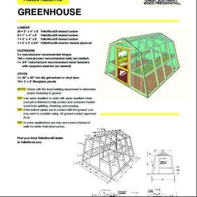
Yellawood Greenhouse Design Plans 4e3y4a
December 2019 59
Automated Greenhouse Monitoring And Control System.pdf o2v1b
October 2019 47
Ngma (greenhouse) Structural Design Manual 328
October 2021 0
Greenhouse-technology-and-management.pdf 1yl6c
October 2022 0
Greenhouse Functions And Controls 4a5a3q
November 2022 0More Documents from "Armando Alvarado Araujo" 36253c
Greenhouse Design And Control By Pedro Ponce 2i6d33
October 2022 0
Taller Lineas Del Tiempo Historia De La Salud Ocupacional En El Mundo Y En Colombia (1).pdf 42571v
May 2021 0
Defectos En La Madera 2r3616
June 2022 0
La Estructura Cognitiva Como Base De La Teoria De Ausubel 273q5e
June 2021 0
504uu
April 2023 0