Tutorial 4z844
This document was ed by and they confirmed that they have the permission to share it. If you are author or own the copyright of this book, please report to us by using this report form. Report 445h4w
Overview 1s532p
& View Tutorial as PDF for free.
More details 6h715l
- Words: 11,473
- Pages: 46
6
Processing Modflow
2. Your First Groundwater Model with PMWIN It takes just a few minutes to build your first groundwater flow model with PMWIN. First, create a groundwater model by choosing New Model from the File menu. Next, determine the size of the model grid by choosing Mesh Size from the Grid menu. Then, specify the geometry of the model and set the model parameters, such as hydraulic conductivity, effective porosity etc.. Finally, perform the flow simulation by choosing MODFLOW<
Overview of the Sample Problem As shown in Fig. 2.1, an aquifer system with two stratigraphic units is bounded by no-flow boundaries on the North and South sides. The West and East sides are bounded by rivers, which are in full hydraulic with the aquifer and can be considered as fixed-head boundaries. The hydraulic heads on the west and east boundaries are 9 m and 8 m above reference level, respectively. The aquifer system is unconfined and isotropic. The horizontal hydraulic conductivities of the first and second stratigraphic units are 0.0001 m/s and 0.0005 m/s, respectively. Vertical hydraulic conductivity of both units is assumed to be 10 percent of the horizontal hydraulic conductivity. The effective porosity is 25 percent. The elevation of the ground surface (top of the first stratigraphic unit) is 10m. The thickness of the first and the second units is 4 m and 6 m, respectively. A constant recharge rate of 8×10⁻⁹ m/s is applied to the aquifer. A contaminated area lies in the first unit next to the west boundary. The task is to isolate the contaminated area using a full penetrated pumping well located next to the eastern boundary. A numerical model has to be developed for this site to calculate the required pumping rate of the well. The pumping rate must be high enough, so that the contaminated area lies within the 2. Your First Groundwater Model with PMWIN
Processing Modflow
7
capture zone of the pumping well. We will use PMWIN to construct the numerical model and use PMPATH to compute the capture zone of the pumping well. Based on the calculated groundwater flow field, we will use MT3D and MOC3D to simulate the contaminant transport. We will show how to use PEST and UCODE to calibrate the flow model and finally we will create an animation sequence displaying the development of the contaminant plume. To demonstrate the use of the transport models, we assume that the pollutant is dissolved into groundwater at a rate of 1×10⁻⁴ µg/s/m 2. The longitudinal and transverse dispersivities of the aquifer are 10m and 1m, respectively. The retardation factor is 2. The initial concentration, molecular diffusion coefficient, and decay rate are assumed to be zero. We will calculate the concentration distribution after a simulation time of 3 years and display the breakthrough curves (concentration versus time) at two points [X, Y] = [290, 310], [390, 310] in both units.
Fig. 2.1 Configuration of the sample problem
2.1 Run a Steady-State Flow Simulation Six main steps must be performed in a steady-state flow simulation: 1. Create a new model model 2. Assign model data 3. Perform the flow simulation 4. Check simulation results 5. Calculate subregional water budget 6. Produce output 2.1 Run a Steady-State Flow Simulation
8
Processing Modflow
Step 1: Create a New Model The first step in running a flow simulation is to create a new model. < 1.
2.
To create a new model Choose New Model from the File menu. A New Model dialog box appears. Select a folder for saving the model data, such as C:\PM5DATA\SAMPLE, and type the file name SAMPLE for the sample model. A model must always have the file extension .PM5. All file names valid under Windows 95/98/NT with up to 120 characters can be used. It is a good idea to save every model in a separate folder, where the model and its output data will be kept. This will also allow you to run several models simultaneously (multitasking). Click OK. PMWIN takes a few seconds to create the new model. The name of the new model name is shown in the title bar.
Step 2: Assign Model Data The second step in running a flow simulation is to generate the model grid (mesh), specify boundary conditions, and assign model parameters to the model grid. PMWIN requires the use of consistent units throughout the modeling process. For example, if you are using length [L] units of meters and time [T] units of seconds, hydraulic conductivity will be expressed in units of [m/s], pumping rates will be in units of [m3/s] and dispersivities will be in units of [m]. In MODFLOW, an aquifer system is replaced by a discretized domain consisting of an array of nodes and associated finite difference blocks (cells). Fig. 2.2 shows a spatial discretization of an aquifer system with a mesh of cells and nodes at which hydraulic heads are calculated. The nodal grid forms the framework of the numerical model. Hydrostratigraphic units can be represented by one or more model layers. The thicknesses of each model cell and the width of each column and row may be variable. The locations of cells are described in of columns, rows, and layers. PMWIN uses an index notation [J, I, K] for locating the cells. For example, the cell located in the 2nd column, 6th row, and the first layer is denoted by [2, 6, 1]. < 1. 2.
To generate the model grid Choose Mesh Size from the Grid menu. The Model Dimension dialog box appears (Fig. 2.3). Enter 3 for the number of layers, 30 for the numbers of columns and rows, and 20 for the size of columns and rows.
2.1 Run a Steady-State Flow Simulation
Processing Modflow
3.
4.
9
The first and second stratigraphic units will be represented by one and two model layers, respectively. Click OK. PMWIN changes the pull-down menus and displays the generated model grid (Fig. 2.4). PMWIN allows you to shift or rotate the model grid, change the width of each model column or row, or to add/delete model columns or rows. For our sample problem, you do not need to modify the model grid. See section 3.1 for more information about the Grid Editor. Choose Leave Editor from the File menu or click the leave editor button
.
Fig. 2.2 Spatial discretization of an aquifer system and the cell indices
Fig. 2.3 The Model Dimension dialog box
2.1 Run a Steady-State Flow Simulation
10
Processing Modflow
Fig. 2.4 The generated model grid
The next step is to specify the type of layers. < To assign the type of layers 1. Choose Layer Type from the Grid menu. A Layer Options dialog box appears. 2. Click a cell of the Type column, a drop-down button will appear within the cell. By clicking the drop-down button, a list containing the avaliable layer types (Fig. 2.5) will be displayed. 3. Select 1: Unconfined for the first layer and 0: Confined for the other layers then click OK to close the dialog box.
Fig. 2.5 The Layer Options dialog box and the layer type drop-down list 2.1 Run a Steady-State Flow Simulation
Processing Modflow
11
Now, you must specify basic boundary conditions of the flow model. The basic boundary contition array (IBOUND array) contains a code for each model cell which indicates whether (1) the hydraulic head is computed (active variable-head cell or active cell), (2) the hydraulic head is kept fixed at a given value (fixed-head cell or time-varying specified-head cell), or (3) no flow takes place within the cell (inactive cell). Use 1 for an active cell, -1 for a constant-head cell, and 0 for an inactive cell. For the sample problem, we need to assign -1 to the cells on the west and east boundaries and 1 to all other cells. < 1.
To assign the boundary condition to the flow model Choose Boundary Condition < IBOUND (Modflow) from the Grid Menu. The Data Editor of PMWIN appears with a plan view of the model grid (Fig. 2.6). The grid cursor is located at the cell [1, 1, 1], that is the upper-left cell of the first layer. The value of the current cell is shown at the bottom of the status bar. The default value of the IBOUND array is 1. The grid cursor can be moved horizontally by using the arrow keys or by clicking the mouse on the desired position. To move to an other layer, use PgUp or PgDn keys or click the edit field in the tool bar, type the new layer number, and then press enter.
Note that a DXF-map is loaded by using the Maps Options. See Chapter 3 for details. 2. 3.
Press the right mouse button. PMWIN shows a Cell Value dialog box. Type -1 in the dialog box, then click OK. The upper-left cell of the model has been specified to be a fixed-head cell.
4.
Now turn on duplication by clicking the duplication button
5.
6. 7. 8.
.
Duplication is on, if the relief of the duplication button is sunk. The current cell value will be duplicated to all cells ed by the grid cursor, if it is moved while duplication is on. You can turn off duplication by clicking the duplication button again. Move the grid cursor from the upper-left cell [1, 1, 1] to the lower-left cell [1, 30, 1] of the model grid. The value of -1 is duplicated to all cells on the west side of the model. Move the grid cursor to the upper-right cell [30, 1, 1]. Move the grid cursor from the upper-right cell [30, 1, 1] to the lower-right cell [30, 30, 1]. The value of -1 is duplicated to all cells on the east side of the model. Turn on layer copy by clicking the layer copy button
.
Layer copy is on, if the relief of the layer copy button is sunk. The cell values of the current layer will be copied to other layers, if you move to the other model layer while layer copy is on. You can turn off layer copy by clicking the layer copy button again. 2.1 Run a Steady-State Flow Simulation
12 9.
Processing Modflow Move to the second layer and then to the third layer by pressing the PgDn key twice. The cell values of the first layer are copied to the second and third layers.
10. Choose Leave Editor from the File menu or click the leave editor button
.
Fig. 2.6 Data Editor with a plan view of the model grid. The next step is to specify the geometry of the model. < To specify the elevation of the top of model layers 1. Choose Top of Layers (TOP) from the Grid menu. PMWIN displays the model grid. 2. Choose Reset Matrix... from the Value menu (or press Ctrl+R). A Reset Matrix dialog box appears. 3. Enter 10 in the dialog box, then click OK. The elevation of the top of the first layer is set to 10. 4. Move to the second layer by pressing PgDn. 5. Repeat steps 2 and 3 to set the top elevation of the second layer to 6 and the top elevation of the third layer to 3. 6.
Choose Leave Editor from the File menu or click the leave editor button
< 1.
To specify the elevation of the bottom of model layers Choose Bottom of Layers (BOT) from the Grid menu.
2.1 Run a Steady-State Flow Simulation
.
Processing Modflow
13
2.
Repeat the same procedure as described above to set the bottom elevation of the first, second and third layers to 6, 3 and 0, respectively.
3.
Choose Leave Editor from the File menu or click the leave editor button
.
We are going to specify the temporal and spatial parameters of the model. The spatial parameters for sample problem include the initial hydraulic head, horizontal and vertical hydraulic conductivities and effective porosity. < 1.
2. 3.
To specify the temporal parameters Choose Time... from the Parameters menu. A Time Parameters dialog box will come up. The temporal parameters include the time unit and the numbers of stress periods, time steps and transport steps. In MODFLOW, the simulation time is divided into stress periods - i.e., time intervals during which all external excitations or stresses are constant - which are, in turn, divided into time steps. In most transport models, each flow time step is further divided into smaller transport steps. The length of stress periods is not relevant to a steady state flow simulation. However, as we want to perform contaminant transport simulation with MT3D and MOC3D, the actual time length must be specified in the table. Enter 9.46728E+07 (seconds) for Length of the first period. Click OK to accept the other default values.
Now, you need to specify the initial hydraulic head for each model cell. The initial hydraulic head at a fixed-head boundary will be kept constant during the flow simulation. The other heads are starting values in a transient simulation or first guesses for the iterative solver in a steadystate simulation. Here we firstly set all values to 8 and then correct the values on the west side by overwriting them with a value of 9. < 1.
3. 4.
To specify the initial hydraulic head Choose Initial Hydraulic Heads from the Parameters menu. PMWIN displays the model grid. Choose Reset Matrix... from the Value menu (or press Ctrl+R) and enter 8 in the dialog box, then click OK. Move the grid cursor to the upper-left model cell. Press the right mouse button and enter 9 into the Cell Value dialog box, then click OK.
5.
Now turn on duplication by clicking the duplication button
2.
.
Duplication is on, if the relief of the duplication button is sunk. The current cell value will 2.1 Run a Steady-State Flow Simulation
14
Processing Modflow
6.
be duplicated to all cells ed over by the grid cursor, if duplication is on. Move the grid cursor from the upper-left cell to the lower-left cell of the model grid. The value of 9 is duplicated to all cells on the west side of the model.
7.
Turn on layer copy by clicking the layer copy button
8.
.
Layer copy is on, if the relief of the layer copy button is sunk. The cell values of the current layer will be copied to another layer, if you move to the other model layer while layer copy is on. Move to the second layer and the third layer by pressing PgDn twice. The cell values of the first layer are copied to the second and third layers.
9.
Choose Leave Editor from the File menu or click the leave editor button
< 1. 2.
5.
To specify the horizontal hydraulic conductivity Choose Horizontal Hydraulic Conductivity from the Parameters menu. Choose Reset Matrix... from the Value menu (or press Ctrl+R), type 0.0001 in the dialog box, then click OK. Move to the second layer by pressing PgDn. Choose Reset Matrix... from the Value menu (or press Ctrl+R), type 0.0005 in the dialog box, then click OK. Repeat steps 3 and 4 to set the value of the third layer to 0.0005.
6.
Choose Leave Editor from the File menu or click the leave editor button
< 1. 2.
5.
To specify the vertical hydraulic conductivity Choose Vertical Hydraulic Conductivity from the Parameters menu. Choose Reset Matrix... from the Value menu (or press Ctrl+R), type 0.00001 in the dialog box, then click OK. Move to the second layer by pressing PgDn. Choose Reset Matrix... from the Value menu (or press Ctrl+R), type 0.00005 in the dialog box, then click OK. Repeat steps 3 and 4 to set the value of the third layer to 0.00005.
6.
Choose Leave Editor from the File menu or click the leave editor button
< 1.
To specify the effective porosity Choose Effective Porosity from the Parameters menu. Because the standard value is the same as the prescribed value of 0.25, you may leave the editor and save the changes.
3. 4.
3. 4.
2.1 Run a Steady-State Flow Simulation
.
.
.
Processing Modflow
15
2.
Choose Leave Editor from the File menu or click the leave editor button
.
< 1. 2.
To specify the recharge rate Choose MODFLOW< < Recharge from the Models menu. Choose Reset Matrix... from the Value menu (or press Ctrl+R), enter 8E-9 for Recharge Flux [L/T] in the dialog box, then click OK.
3.
Choose Leave Editor from the File menu or click the leave editor button
.
The last step before performing the flow simulation is to specify the location of the pumping well and its pumping rate. In MODFLOW, an injection or pumping well is represented by a node (or a cell). The specifies an injection or pumping rate for each node. It is implicitly assumed that the well penetrates the full thickness of the cell. MODFLOW can simulate the effects of pumping from a well that penetrates more than one aquifer or layer provided that the supplies the pumping rate for each layer. The total pumping rate for the multilayer well is equal to the sum of the pumping rates from the individual layers. The pumping rate for each layer ( Qk ) can be approximately calculated by dividing the total pumping rate ( Qtotal ) in proportion to the layer transmissivities (McDonald and Harbaugh, 1988): Qk ' Qtotal @
Tk
(2.1)
ET
where TKk is the transmissivity of layer k and ET is the sum of the transmissivities of all layers penetrated by the multilayer well. Unfortunately, as the first layer is unconfined, we do not exactly know the saturated thickness and the transmissivity of this layer at the position of the well. Eq. 2.1 cannot be used unless we assume a saturated thickness for calculating the transmissivity. An other possibility to simulate a multi-layer well is to set a very large vertical hydraulic conductivity (or vertical leakance), e.g. 1 m/s, to all cells of the well. The total pumping rate is assigned to the lowerst cell of the well. For the display purpose, a very small pumping rate (say, 1×10⁻¹⁰ m3/s) can be assigned to other cells of the well. In this way, the exact extraction rate from each penetrated layer will be calculated by MODFLOW implicitly and the value can be obtained by using the Water Budget Calculator (see below). As we do not know the required pumping rate for capturing the contaminated area shown in Fig. 2.1, we will try a total pumping rate of 0.0012 m3/s. < 1. 2.
To specify the pumping well and the pumping rate Choose MODFLOW< <Well from the Models menu. Move the grid cursor to the cell [25, 15, 1] 2.1 Run a Steady-State Flow Simulation
16
Processing Modflow
3. 4. 5. 6. 7.
Press the right mouse button and type -1E-10, then click OK. Note that a negative value is used to indicate a pumping well. Move to the second layer by pressing PgDn. Press the right mouse button and type -1E-10 then click OK. Move to the third layer by pressing PgDn. Press the right mouse button and type -0.0012 then click OK.
8.
Choose Leave Editor from the File menu or click the leave editor button
.
Step 3: Perform the Flow Simulation < To perform the flow simulation 1. Choose MODFLOW<
Fig. 2.7 The Run Modflow dialog box Step 4: Check Simulation Results During a flow simulation, MODFLOW writes a detailed run record to the listing file path\OUTPUT.DAT, where path is the folder in which your model data are saved. If a flow 2.1 Run a Steady-State Flow Simulation
Processing Modflow
17
simulation is successfully completed, MODFLOW saves the simulation results in various unformatted (binary) files as listed in Table 2.1. Prior to running MODFLOW, the may control the output of these unformatted (binary) files by choosing Modflow<
Contents
path\OUTPUT.DAT
Detailed run record and simulation report
path\HEADS.DAT
Hydraulic heads
path\DDOWN.DAT
Drawdowns, the difference between the starting heads and the calculated hydraulic heads.
path\BUDGET.DAT
Cell-by-Cell flow
path\INTERBED.DAT
Subsidence of the entire aquifer and compaction and preconsolidation heads in individual layers.
path\MT3D.FLO
Interface file to MT3D/MT3DMS. This file is created by the LKMT package provided by MT3D/MT3DMS (Zheng, 1990, 1998).
- path is the folder in which the model data are saved.
2.1 Run a Steady-State Flow Simulation
18
Processing Modflow
Table 2.2 Volumetric budget for the entire model written by MODFLOW VOLUMETRIC BUDGET FOR ENTIRE MODEL AT END OF TIME STEP 1 IN STRESS PERIOD 1 ----------------------------------------------------------------------------CUMULATIVE VOLUMES -----------------IN: --CONSTANT HEAD = WELLS = RECHARGE = TOTAL IN =
L**3
RATES FOR THIS TIME STEP ------------------------
L**3/T
209690.3590 0.0000 254472.9380
IN: --CONSTANT HEAD = WELLS = RECHARGE =
2.2150E-03 0.0000 2.6880E-03
464163.3130
TOTAL IN =
4.9030E-03
OUT: ---CONSTANT HEAD = WELLS = RECHARGE =
350533.6880 113604.0310 0.0000
OUT: ---CONSTANT HEAD = WELLS = RECHARGE =
3.7027E-03 1.2000E-03 0.0000
TOTAL OUT =
464137.7190
TOTAL OUT =
4.9027E-03
IN - OUT =
25.5938
IN - OUT =
2.7008E-07
PERCENT DISCREPANCY =
0.01
PERCENT DISCREPANCY =
0.01
Step 5: Calculate subregional water budget There are situations in which it is useful to calculate water budgets for various subregions of the model. To facilitate such calculations, flow for individual cells are saved in the file path\BUDGET.DAT. These individual cell flows are referred to as cell-by-cell flow , and are of four types: (1) cell-by-cell stress flows, or flows into or from an individual cell due to one of the external stresses (excitations) represented in the model, e.g., pumping well or recharge; (2) cell-by-cell storage , which give the rate of accumulation or depletion of storage in an individual cell; (3) cell-by-cell constant-head flow , which give the net flow to or from individual fixed-head cells; and (4) internal cell-by-cell flows, which are the flows across individual cell faces-that is, between adjacent model cells. The Water Budget Calculator uses the cell-by-cell flow to compute water budgets for the entire model, -specified subregions, and flows between adjacent subregions. < 1.
2.
To calculate subregional water budgets Choose Water Budget from the Tools menu. A Water Budget dialog box appears (Fig. 2.8). For a steady-state flow simulation, you do not need to change the settings in the Time group. Click Zones. A zone is a subregion of a model for which a water budget will be calculated. A zone is indicated by a zone number ranging from 0 to 50. A zone number must be assigned to each model cell. The zone number 0 indicates that a cell is not associated with any zone. Follow
2.1 Run a Steady-State Flow Simulation
Processing Modflow
19
3. 4. 5.
steps 3 to 5 to assign zone numbers 1 to the first and 2 to the second layer. Choose Reset Matrix... from the Value menu, type 1 in the dialog box, then click OK. Press PgDn to move to the second layer. Choose Reset Matrix... from the Value menu, type 2 in the dialog box, then click OK.
6.
Choose Leave Editor from the File menu or click the leave editor button
7.
Click OK in the Water Budget dialog box.
.
Fig. 2.8 The Water Budget dialog box PMWIN calculates and saves the flows in the file path\WATERBDG.DAT as shown in Table 2.3. The unit of the flows is [L3T-1]. Flows are calculated for each zone in each layer and each time step. Flows are considered IN, if they are entering a zone. Flows between subregions are given in a Flow Matrix. HORIZ. EXCHANGE gives the flow rate horizontally across the boundary of a zone. EXCHANGE (UPPER) gives the flow rate coming from (IN) or going to (OUT) to the upper adjacent layer. EXCHANGE (LOWER) gives the flow rate coming from (IN) or going to (OUT) to the lower adjacent layer. For example, consider EXCHANGE (LOWER) of ZONE=1 and LAYER=1, the flow rate from the first layer to the second layer is 2.587256E-03 m3/s. The percent discrepancy in Table 2.3 is calculated by
100 @ (IN & OUT) (IN % OUT) / 2
(2.2)
In this example, the percent discrepanciy of in- and outflows for the model and each zone in each layer is acceptably small. This means the model equations have been correctly solved. To calculate the exact flow rates to the well, we repeat the previous procedure for calculating subregional water budgets. This time we only assign the cell [25, 15, 1] to zone 1, the cell [25, 15, 2] to zone 2 and the cell [25, 15, 3] to zone 3. All other cells are assigned to zone 0. The water budget is shown in Table 2.4. The pumping well is extracting 7.7992809E-05 m3/s from the first layer, 5.603538E-04 m3/s from the second layer and 5.5766129E-04 m3/s from the third layer. Almost all withdrawn water comes from the second stratigraphic unit, as it 2.1 Run a Steady-State Flow Simulation
20
Processing Modflow
can be expected from the configuration of the aquifer. Table 2.3 Output from the Water Budget Calculator FLOWS ARE CONSIDERED "IN" IF THEY ARE ENTERING A SUBREGION THE UNIT OF THE FLOWS IS [L^3/T] TIME STEP ZONE=
1 OF STRESS PERIOD
1 LAYER= FLOW TERM STORAGE CONSTANT HEAD HORIZ. EXCHANGE EXCHANGE (UPPER) EXCHANGE (LOWER) WELLS DRAINS RECHARGE . . . SUM OF THE LAYER . .
1
1 IN 0.0000000E+00 1.8407618E-04 0.0000000E+00 0.0000000E+00 0.0000000E+00 0.0000000E+00 0.0000000E+00 2.6880163E-03 . . 2.8720924E-03 . .
OUT IN-OUT 0.0000000E+00 0.0000000E+00 2.4361895E-04 -5.9542770E-05 0.0000000E+00 0.0000000E+00 0.0000000E+00 0.0000000E+00 2.5872560E-03 -2.5872560E-03 1.0000000E-10 -1.0000000E-10 0.0000000E+00 0.0000000E+00 0.0000000E+00 2.6880163E-03 . 2.8308749E-03 . .
.
. 4.1217543E-05 . .
ZONE=
2 LAYER= 2 FLOW TERM IN OUT IN-OUT STORAGE 0.0000000E+00 0.0000000E+00 0.0000000E+00 CONSTANT HEAD 1.0027100E-03 1.7383324E-03 -7.3562248E-04 HORIZ. EXCHANGE 0.0000000E+00 0.0000000E+00 0.0000000E+00 EXCHANGE (UPPER) 2.5872560E-03 0.0000000E+00 2.5872560E-03 EXCHANGE (LOWER) 0.0000000E+00 1.8930938E-03 -1.8930938E-03 WELLS 0.0000000E+00 1.0000000E-10 -1.0000000E-10 DRAINS 0.0000000E+00 0.0000000E+00 0.0000000E+00 RECHARGE 0.0000000E+00 0.0000000E+00 0.0000000E+00 . . . . . . . SUM OF THE LAYER 3.5899659E-03 3.6314263E-03 -4.1460386E-05 -------------------------------------------------------------. . . . . . . . WATER BUDGET OF SELECTED ZONES: IN OUT IN-OUT ZONE( 1): 2.8720924E-03 2.8308751E-03 4.1217310E-05 ZONE( 2): 3.5899659E-03 3.6314263E-03 -4.1460386E-05 -------------------------------------------------------------WATER BUDGET OF THE WHOLE MODEL DOMAIN: FLOW TERM IN OUT IN-OUT STORAGE 0.0000000E+00 0.0000000E+00 0.0000000E+00 CONSTANT HEAD 2.2149608E-03 3.7026911E-03 -1.4877303E-03 WELLS 0.0000000E+00 1.2000003E-03 -1.2000003E-03 DRAINS 0.0000000E+00 0.0000000E+00 0.0000000E+00 RECHARGE 2.6880163E-03 0.0000000E+00 2.6880163E-03 . . . . . . . . -------------------------------------------------------------SUM 4.9029770E-03 4.9026916E-03 2.8545037E-07 DISCREPANCY [%] 0.01 The value of the element (i,j) of the following flow matrix gives the flow rate from the i-th zone into the j-th zone. Where i is the column index and j is the row index. FLOW MATRIX: 1 2 ............................. 0 1 0.0000 0.0000 0 2 2.5873E-03 0.0000
2.1 Run a Steady-State Flow Simulation
.
Processing Modflow
21
Table 2.4 Output from the Water Budget Calculator for the pumping well FLOWS ARE CONSIDERED "IN" IF THEY ARE ENTERING A SUBREGION THE UNIT OF THE FLOWS IS [L^3/T] TIME STEP 1 OF ZONE= 1 LAYER= FLOW TERM STORAGE CONSTANT HEAD HORIZ. EXCHANGE EXCHANGE (UPPER) EXCHANGE (LOWER) WELLS DRAINS RECHARGE . . SUM OF THE LAYER . . ZONE= 2 LAYER= FLOW TERM STORAGE CONSTANT HEAD HORIZ. EXCHANGE EXCHANGE (UPPER) EXCHANGE (LOWER) WELLS . . SUM OF THE LAYER ZONE=
3 LAYER= FLOW TERM STORAGE CONSTANT HEAD HORIZ. EXCHANGE EXCHANGE (UPPER) EXCHANGE (LOWER) WELLS . . SUM OF THE LAYER
STRESS PERIOD 1 IN 0.0000000E+00 0.0000000E+00 7.7992809E-05 0.0000000E+00 0.0000000E+00 0.0000000E+00 0.0000000E+00 3.1999998E-06 . . 8.1192811E-05 . . 2 IN 0.0000000E+00 0.0000000E+00 5.6035380E-04 7.9696278E-05 0.0000000E+00 0.0000000E+00 . . 6.4005010E-04
1 OUT IN-OUT 0.0000000E+00 0.0000000E+00 0.0000000E+00 0.0000000E+00 0.0000000E+00 7.7992809E-05 0.0000000E+00 0.0000000E+00 7.9696278E-05 -7.9696278E-05 1.0000000E-10 -1.0000000E-10 0.0000000E+00 0.0000000E+00 0.0000000E+00 3.1999998E-06 . . . . 7.9696380E-05 1.4964317E-06 . . . . OUT IN-OUT 0.0000000E+00 0.0000000E+00 0.0000000E+00 0.0000000E+00 0.0000000E+00 5.6035380E-04 0.0000000E+00 7.9696278E-05 6.4027577E-04 -6.4027577E-04 1.0000000E-10 -1.0000000E-10 . . . . 6.4027589E-04 -2.2578752E-07
3 IN 0.0000000E+00 0.0000000E+00 5.5766129E-04 6.4027577E-04 0.0000000E+00 0.0000000E+00 . . 1.1979371E-03
OUT IN-OUT 0.0000000E+00 0.0000000E+00 0.0000000E+00 0.0000000E+00 0.0000000E+00 5.5766129E-04 0.0000000E+00 6.4027577E-04 0.0000000E+00 0.0000000E+00 1.2000001E-03 -1.2000001E-03 . . . . 1.2000001E-03 -2.0629959E-06
Step 6: Produce Output In addition to the water budget, PMWIN provides various possibilities for checking simulation results and creating graphical outputs. Pathlines and velocity vectors can be displayed by PMPATH. Using the Results Extractor, simulation results of any layer and time step can be read from the unformatted (binary) result files and saved in ASCII Matrix files. An ASCII Matrix file contains a value for each model cell in a layer. PMWIN can load ASCII matrix files into a model grid. The format of the ASCII Matrix file is described in Appendix 2. In the following, we will carry out the steps: 1. Use the Results Extractor to read and save the calculated hydraulic heads. 2. Generate a contour map based on the calculated hydraulic heads for the first layer. 3. Use PMPATH to compute pathlines as well as the capture zone of the pumping well.
2.1 Run a Steady-State Flow Simulation
22
Processing Modflow
< 1.
To read and save the calculated hydraulic heads Choose Results Extractor... from the Tools menu The Results Extractor dialog box appears (Fig. 2.9). The options in the Results Extractor dialog box are grouped under four tabs - MODFLOW, MOC3D, MT3D and MT3DMS. In the MODFLOW tab, you may choose a result type from the Result Type drop-down box. You may specify the layer, stress period and time step from which the result should be read. The spreadsheet displays a series of columns and rows. The intersection of a row and column is a cell. Each cell of the spreadsheet corresponds to a model cell in a layer. Refer to Chap. 5 for more detailed information about the Results Extractor. For the current sample problem, follow steps 2 to 6 to save the hydraulic heads of each layer in three ASCII Matrix files. Choose Hydraulic Head from the Result Type drop-down box. Type 1 in the Layer edit field. For the current problem (steady-state flow simulation with only one stress period and one time step), the stress period and time step number should be 1. Click Read. Hydraulic heads in the first layer at time step 1 and stress period 1 will be read and put into the spreadsheet. You can scroll the spreadsheet by clicking on the scrolling bars next to the spreadsheet. Click Save. A Save Matrix As dialog box appears. By setting the Save as type option, the result can be optionally saved as an ASCII matrix or a SURFER data file. Specify the file name H1.DAT and select a folder in which H1.DAT should be saved. Click OK when ready. Repeat steps 3, 4 and 5 to save the hydraulic heads of the second and third layer in the files H2.DAT and H3.DAT, respectively. Click Close to close the dialog box.
2. 3.
4.
5.
6. 7. < 1.
2.
To generate contour maps of the calculated heads Choose Presentation from the Tools menu Data specified in Presentation will not be used by any parts of PMWIN. We can use Presentation to save temporary data or to display simulation results graphically. Choose Matrix... from the Value menu (or Press Ctrl+B). The Browse Matrix dialog box appears (Fig. 2.10). Each cell of the spreadsheet corresponds to a model cell in the current layer. You can load an ASCII Matrix file into the spreadsheet or save the spreadsheet in an ASCII Matrix file by clicking Load or Save. Alternatively, you may select the Results Extractor from the Value menu, read the head
2.1 Run a Steady-State Flow Simulation
Processing Modflow
3. 4. 5. 6.
7.
23
results and use an additional Apply button in the Results Extractor dialog box to put the data into the Presentation matrix. Click the Load... button. The Load Matrix dialog box appears (Fig. 2.11). Click
and select the file H1.DAT, which was saved earlier by the Results Extractor.
Click OK when ready. H1.DAT is loaded into the spreadsheet. In the Browse Matrix dialog box, click OK. The Browse Matrix dialog box is closed. Choose Environment from the Options menu (or Press Ctrl+E). The Environment Options dialog box appears (Fig. 2.12). The options in the Environment Options dialog box are grouped under three tabs. Appearance and Coordinate System allow the to modify the appearance and position of the model grid. Use Contours to generate contour maps. Click the Contours tab, check Visible, then click the Restore Defaults button. Clicking on the Restore Defaults button, PMWIN sets the number of contour lines to 11 and uses the maxmum and minimum values in the current layer as the minimum and maximum contour levels (Fig. 2.13). If Fill Contours is checked, the contours will be filled with the colors given in the Fill column of the table. Use Label Format button to specify an appropriate format.
Note that PMWIN will clear the Visible check box when you leave the Editor. 8.
In the Environment Options dialog box, Click OK. PMWIN will redraw the model and display the contours (Fig. 2.14). 9. To save or print the graphics, choose Save Plot As... or Print Plot... from the File menu. 10. Press PgDn to move to the second layer. Repeat steps 2 to 9 to load the file H2.DAT, display and save the plot. 11. Choose Leave Editor from the File menu or click the leave editor button
and click Yes
to save changes to Presentation. Using the foregoing procedure, you can generate contour maps based on your input data, any kind of simulation results or any data saved as an ASCII Matrix file. For example, you can create a contour map of the starting heads or you can use the Result Extractor to read the concentration distribution and display the contours. You can also generate contour maps of the fields created by the Field Interpolator or Field Generator. See chapter 5 for details about the Field Interpolator and Field Generator.
2.1 Run a Steady-State Flow Simulation
24
Processing Modflow
Fig. 2.9 The Results Extractor dialog box.
Fig. 2.10 The Browse Matrix dialog box
Fig. 2.11 The Load Matrix dialog box
2.1 Run a Steady-State Flow Simulation
Processing Modflow
25
Fig. 2.12 The Environment Options dialog box
Fig. 2.13 The Contours options of the Environment Options dialog box
2.1 Run a Steady-State Flow Simulation
26
Processing Modflow
Fig. 2.14 A contour map of the hydraulic heads in the first layer < 1.
To delineate the capture zone of the pumping well Choose PMPATH (Pathlines and Contours) from the Models menu. PMWIN calls the advective transport model PMPATH and the current model will be loaded into PMPATH automatically. PMPATH uses a "grid cursor" to define the column and row for which the cross-sectional plots should be displayed. You can move the grid cursor by holding down the Ctrl-key and click the left mouse button on the desired position.
Note that if you subseguently modify and calculate a model within PMWIN, you must load the modified model into PMPATH again to ensure that the modifications can be recongnized by PMPATH. To load a model, click and select a model file with the extension .PM5 from the Open Model dialog box.
2. To calculate the capture zone of the pumping well: a. Click the Set Particle button b. Move the mouse cursor to the model area. The mouse cursor turns into crosshairs. c. Place the crosshairs at the upper-left corner of the pumping well, as shown in Fig. 2.15. d. Hold down the left moust button and drag the crosshairs until the window covers the pumping well. e. Release the left mouse button. An Add New Particles dialog box appears. Assign the numbers of particles to the edit 2.1 Run a Steady-State Flow Simulation
Processing Modflow
27
fields in the dialog box as shown in Fig. 2.16. Click the Properties tab and click the colored button to select an appropriate color for the new particles. When finished, click OK. f. To set particles around the pumping well in the second and third layer, press PgDn to move down a layer and repeat steps c, d and e. Use other colors for the new particles in the second and third layers. g. Click
to start the backward particle tracking.
PMPATH calculates and shows the projections of the pathlines as well as the capture zone of the pumping well (Fig. 2.17). To see the projection of the pathlines on the cross-section windows in greater details, open an Environment Options dialog box by choosing Environment... from the Options menu and set a larger exaggeration value in the Cross Sections tab. Fig. 2.18 shows the same pathlines by setting the exaggeration value to 10. Note that some pathlines end up at the groundwater surface, where recharge occurs. This is one of the major differences between a threedimensional and a two-dimensional model. In two-dimensional areal simulation models, such as ASM for Windows (Chiang et al., 1998), FINEM (Kinzelbach et al, 1990) or MOC (Konikow and Bredehoeft, 1978), a vertical velocity term does not exist (or always equals to zero). This leads to the result that pathlines can never be tracked back to the ground surface where the groundwater recharge from the precipitation occurs. PMPATH can create time-related capture zones of pumping wells. The 100-days-capture zone shown in Fig. 2.19 is created by using the settings in the Particle Tracking (Time) Properties dialog box (Fig. 2.20) and clicking
. To open this dialog box, choose Particle
Tracking (Time)... from the Options menu. Note that because of lower hydraulic conductivity (and thus lower flow velocity) the capture zone in the first layer is smaller than those in the other layers.
2.1 Run a Steady-State Flow Simulation
28
Processing Modflow
Fig. 2.15 The sample model loaded in PMPATH
Fig. 2.16 The Add New Particles dialog box
2.1 Run a Steady-State Flow Simulation
Processing Modflow
29
Fig. 2.17 The capture zone of the pumping well (with vertical exaggeration=1)
Fig. 2.18 The capture zone of the pumping well (with vertical exaggeration=10)
2.1 Run a Steady-State Flow Simulation
30
Processing Modflow
Fig. 2.19 100-days-capture zone calculated by PMPATH
Fig. 2.20 The Particle Tracking (Time) Properties dialog box
2.1 Run a Steady-State Flow Simulation
Processing Modflow
31
2.2 Simulation of Solute Transport Basically, the transport of solutes in porous media can be described by three processes: advection, hydrodynamic dispersion and physical, chemical or biochemical reactions. Both the MT3D and MOC3D models use the method-of-characteristics (MOC) to simulate the advection transport, in which dissolved chemicals are represented by a number of particles and the particles are moving with the flowing groundwater. Besides the MOC method, the MT3D and MT3DMS models provide other methods for solving the advective term, see sections 3.6.3 and 3.6.4 for details. The hydrodynamic dispersion can be expressed in of the dispersivity [L] and the coefficient of molecular diffusion [L2T-1] for the solute in the porous medium. The types of reactions incorporated into MOC3D are restricted to those that can be represented by a firstorder rate reaction, such as radioactive decay, or by a retardation factor, such as instaneous, reversible, sorption-desorption reactions goverened by a linear isotherm and constant distribution coefficient (Kd). In addition to the linear isotherm, MT3D s non-linear isotherms, i.e., Freundlich and Langmuir isotherms. Prior to running MT3D or MOC3D, you need to define the observation boreholes, for which the breakthrough curvers will be calculated. < To define observation boreholes 1. Choose Boreholes and Observations from the Paramters menu. A Boreholes and Observations dialog box appears. Enter the coordinates of the observation boreholes into the dialog box as shown in Fig. 2.21. 2. Click OK to close the dialog box.
Fig. 2.21 The Boreholes and Observations dialog box 2.2 Simulation of Solute Transport
32
Processing Modflow
2.2.1 Perform Transport Simulation with MT3D MT3D requires a boundary condition code for each model cell which indicates whether (1) solute concentration varies with time (active concentration cell), (2) the concentration is kept fixed at a constant value (constant-concentration cell), or (3) the cell is an inactive concentration cell. Use 1 for an active concentration cell, -1 for a constant-concentration cell, and 0 for an inactive concentration cell. Active, variable-head cells can be treated as inactive concentration cells to minimize the area needed for transport simulation, as long as the solute concentration is insignificant near those cells. Similar to the flow model, you must specify the initial concentration for each model cell. The initial concentration at a constant-concentration cell will be kept constant during a transport simulation. The other concentration are starting values in a transport simulation. < 1.
To assign the boundary condition to MT3D Choose Boundary Conditions < ICBUND (MT3D/MT3DMS) from the Grid menu. For the current example, we accept the default value 1 for all cells.
2.
Choose Leave Editor from the File menu or click the leave editor button
< 1.
To set the initial concentration Choose MT3D < Initial Concentration from the Models menu. For the current example, we accept the default value 0 for all cells.
2.
Choose Leave Editor from the File menu or click the leave editor button
< 1. 2.
To assign the input rate of contaminants Choose MT3D < Sink/Source Concentration < Recharge from the Models menu. Assign 12500 [µg/m 3] to the cells within the contaminated area. This value is the concentration associated with the recharge flux. Since the recharge rate is 8 × 10⁻⁹ [m3/m2 /s] and the dissolution rate is 1 × 10⁻⁴ [µg/s/m2 ], the concentration associated with the recharge flux is 1 × 10⁻⁴ / 8 × 10-9 = 12500 [µg/m 3]
3.
Choose Leave Editor from the File menu or click the leave editor button
< 1.
To assign the transport parameters to the Advection Package Choose MT3D < Advection... from the Models menu. An Advection Package (MTADV1) dialog box appears. Enter the values as shown in Fig. 2.22 into the dialog box, select Method of Characteritics (MOC) for the solution scheme and First-order Euler for the particle tracking algorithm.
2.2.1 Perform Transport Simulation with MT3D
.
.
.
Processing Modflow 2.
33
Click OK to close the dialog box.
Fig. 2.22 The Advection Package (MTADV1) dialog box < 1.
2.
3.
To assign the dispersion parameters Choose MT3D < Dispersion... from the Models menu. A Dispersion Package (MT3D) dialog box appears. Enter the ratios of the transverse dispersivity to longitudinal dispersivity as shown in Fig. 2.23. Click OK. PMWIN displays the model grid. At this point you need to specify the longitudinal dispersivity to each cell of the grid. Choose Reset Matrix... from the Value menu (or press Ctrl+R), type 10 in the dialog box then click OK.
4.
Turn on layer copy by clicking the layer copy button
.
5.
Move to the second layer and the third layer by pressing PgDn twice. The cell values of the first layer are copied to the second and third layers.
6.
Choose Leave Editor from the File menu or click the leave editor button
< 1.
To assign the chemical reaction parameters Choose MT3D < Chemical Reaction < Layer by Layer from the Models menu. A Chemical Reaction Package (MTRCT1) dialog box appears. Clear the check box Simulate the radioactive decay or biodegradation and select Linear equlibrium
.
2.2.1 Perform Transport Simulation with MT3D
34
Processing Modflow isotherm for the type of sorption. For the linear isotherm, the retardation factor R for each cell is calculated at the beginning of the simulation by
R ' 1 %
Db n
@ Kd
(2.3)
Where n [-] is the effective porosity with respect to the flow through the porous medium, D b [ML-3] is the bulk density of the porous medium and K d [L M3 ]-1is the distribution coefficient of the solute in the porous medium. As the effective porosity is equal to 0.25, setting Db = 2000 and Kd = 0.000125 yields R = 2. 2.
Click OK to close the Chemical Reaction Package (MTRCT1) dialog box (Fig. 2.24).
The last step before running the transport model is to specify the output times, at which the calculated concentration should be saved. < 1.
2.
3.
To specify the output times Choose MT3D < Output Control... from the Models menu. An Output Control (MT3D, MT3DMS) dialog box appears. The options in this dialog box are grouped under three tabs - Output , Output Times and Misc. Click the Output Times tab, then click the header Output Time of the (empty) table. An Output Times dialog box appears. Enter 3000000 to Interval in this dialog box then click OK to accept the other defalut values. Click OK to close the Output Control (MT3D, MT3DMS) dialog box (Fig. 2.25).
Fig. 2.23 The Advection Package (MTADV1) dialog box
2.2.1 Perform Transport Simulation with MT3D
Processing Modflow
35
Fig. 2.24 The Chemical Reaction Package (MTRCT1) dialog box
Fig. 2.25 The Output Control (MT3D, MT3DMS) dialog box < 1. 2.
To perform the transport simulation Choose MT3D<
2.2.1 Perform Transport Simulation with MT3D
36
Processing Modflow
Fig. 2.26 The Run MT3D/MT3D96 dialog box < Check simulation results and produce output During a transport simulation, MT3D writes a detailed run record to the file path\OUTPUT.MT3, where path is the folder in which your model data are saved. MT3D saves the simulation results in various files, which can be controlled by choosing MT3D < Output Control... from the Models menu. To check the quality of the simulation results, a mass budget is calculated at the end of each transport step and accumulated to provide summarized information on the total mass into or out of the groundwater flow system. The discrepancy between the total mass in and out servers as an indicator of the accuracy of the simulation results. It is highly recommended to check the record file or at least take a glance at it. Using Presentation you can generate contour maps of the calculated concentration. Fig. 2.27 shows the calculated concentration in the third layer at the end of the simulation (simulation time=9.467E+07 seconds). To generate the breakthrough curves, choose Graphs < Concentration Time < MT3D from the Tools menu. Click on the Plot flags of the Boreholes table until they are set to (Fig. 2.28).
2.2.1 Perform Transport Simulation with MT3D
Processing Modflow
37
Fig. 2.27 Simulated concentration at 3 years in the third layer
Fig. 2.28 Concentration-time curves at the observation boreholes
2.2.1 Perform Transport Simulation with MT3D
38
Processing Modflow
2.2.2 Perform Transport Simulation with MOC3D In MOC3D, transport may be simulated within a subgrid, which is a “window” within the primary model grid used to simulate flow. Within the subgrid, the row and column spacing must be uniform, but the thickness can vary from cell to cell and layer to layer. However, the range in thickness values (or product of thickness and effective porosity) should be as small as possible. The initial concentration must be specified throughout the subgrid within which solute transport occurs. MOC3D assumes that the concentration outside of the subgrid is the same within each layer, so only one value is specified for each layer within and adjacent to the subgrid. The use of constant-concentration boundary condition has not been implemented in MOC3D. < 1.
To set the initial concentration Choose MOC3D < Initial Concentration from the Models menu. For the current example, we accept the default value 0 for all cells. Note that PMWIN automatically uses the same initial concentration values for both MOC3D and MT3D.
2.
Choose Leave Editor from the File menu or click the leave editor button
< 1.
To define the transport subgrid and the concentration outside of the subgrid Choose MOC3D < Subgrid... from the Models menu. The Subgrid for Transport (MOC3D) dialog box appears (Fig. 2.29). The options in the dialog box are grouped under two tabs - Subgrid and C’ Outside of Subgrid. The default size of the subgrid is the same as the model grid used to simulate flow. The default initial concentration outside of the subgrid is zero. We will accept the defaults. Click OK to accept the default values and close the dialog box.
2.
Fig. 2.29 The Subgrid for Transport (MOC3D) dialog box.
2.2.2 Perform Transport Simulation with MOC3D
.
Processing Modflow
39
< 1. 2.
To assign the input rate of contaminants Choose MOC3D < Sink/Source Concentration < Recharge from the Models menu. Assign 12500 [µg/m 3] to the cells within the contaminated area. This value is the concentration associated with the recharge flux. Since the recharge rate is 8 × 10⁻⁹ [m3/m2/s] and the dissolution rate is 1 × 10⁻⁴ [µg/s/m2 ], the concentration associated with the recharge flux is 1 × 10⁻⁴ / 8 × 10-9 = 12500 [µg/m 3]
3.
Choose Leave Editor from the File menu or click the leave editor button
< 1.
To assign the parameters for the advective transport Choose MOC3D < Advection... from the Models menu. A Parameters for Advection Transport (MOC3D) dialog box appears. Enter the values as shown in Fig. 2.30 into the dialog box, select Bilinear (X, Y directions) for the interpolation scheme for particle velocity. As noted by Konikow et al. (1996), if transmissivity within a layer is homogeneous or smoothly varying, bilinear interpolation of velocity yields more realistic pathlines for a given discretization than does linear interpolation. Click OK to close the dialog box.
2.
.
Fig. 2.30 The Parameters for Advective Transport dialog box. < 1.
2.
To assign the parameters for dispersion and chemical reaction Choose MOC3D < Dispersion & Chemical Reaction... from the Models menu. A Dispersion / Chemical Reaction (MOC3D) dialog box appears. Check Simulate Dispersion and enter the values as shown in Fig. 2.31. Note that the paramters for dispersion and chemical reaction are the same for each layer. Click OK to close the dialog box.
2.2.2 Perform Transport Simulation with MOC3D
40
Processing Modflow
Fig. 2.31 The Dispersion / Chemical Reaction (MOC3D) dialog box. < 1. 2. 3.
4.
To set Strong/Weak Flag Choose MOC3D < Strong/Weak Flag from the Models menu. Move the grid cursor to the cell [25, 15, 1]. Press the right mouse button and type 1, then click OK. Note that a strong sink or source is indicated by the value of 1 in the matrix. When a fluid source is “strong”, new particles are added to replace old particles as they are advected out of that cell. Where a fluid sink is “strong”, particles are removed after they enter that cell. Repeat steps 2 and 3 to assign the value 1 to the cells [25, 15, 2] and [25, 15, 3].
5.
Choose Leave Editor from the File menu or click the leave editor button
< 1.
To specify the output and times Choose MOC3D < Output Control... from the Models menu. An Output Control (MOC3D) dialog box appears. The options in the dialog box are grouped under five tabs - Concentration, Velocity, Particle Locations, Disp. Coeff. and Misc. In the Concentration tab, select the option These data will be printed or saved every Nth particle moves and enter N = 20. Click OK to accept all other default values and close the Output Control (MOC3D) dialog box (Fig. 2.32).
2. 3.
2.2.2 Perform Transport Simulation with MOC3D
.
Processing Modflow
41
Fig. 2.32 The Output Control (MOC3D) dialog box.
< 1. 2.
To perform the transport simulation Choose MOC3D<
Fig. 2.33 The Run MOC3D dialog box
2.2.2 Perform Transport Simulation with MOC3D
42
Processing Modflow
< Check simulation results and produce output During a transport simulation, MOC3D writes a detailed run record to the file path\MOC3D.LST, where path is the folder in which your model data are saved. MOC3D saves the simulation results in various files, which can be controlled by choosing MOC3D < Output Control... from the Models menu. To check the quality of the simulation results, mass balance calculations are performed and saved in the run record file. The mass in storage at any time is calculated from the concentrations at the nodes of the transport subgrid to provide summarized information on the total mass into or out of the groundwater flow system. The mass balance error will typically exhibit an oscillatory behavior over time, because of the finite-difference approximation and the nature of the method of characteristics. As discussed in Konikow et al. (1996), as long as the oscillations remain within a steady range, not exceeding about ±10 percent as a guide, then the error probably does not represent a bias and is not a serious problem. Rather, the ocillations only reflect the fact the mass balance calculation is itself just an approximation. Using Presentation you can generate contour maps of the calculated concentration. Fig. 2.34 shows the calculated concentration at 3 years in the third layer (simulation time=9.467E+07 seconds). To generate the breakthrough curves, choose Graphs < Concentration Time < MOC3D from the Tools menu. Click on the Plot flags of the Boreholes table until they are set to (Fig. 2.35).
Fig. 2.34 Simulated concentration at 3 years in the third layer 2.2.2 Perform Transport Simulation with MOC3D
Processing Modflow
43
Fig. 2.35 Concentration-time curves at the observation boreholes
2.3 Automatic Calibration Calibration of a flow model is accomplished by finding a set of parameters, hydrologic stresses or boundary conditions so that the simulated heads or drawdowns match the measurement values to a reasonable degree. The calibration process is one of the most difficult and critical steps in the model application. Hill (1998) gives methods and guidelines for modeling calibration using inverse modeling. To demonstrate the use of the inverse models PEST and UCODE within PMWIN, we assume that the hydraulic conductivities in the third layer is homogeneous but its value is unknown. We want to find out this value through a model calibration by using the measured hydraulic heads at the observation boreholes listed below. Borehole
X-coordinate
Y-coordinate
Layer
Hydraulic Head
1
130
200
3
8.85
2
200
400
3
8.74
3
480
250
3
8.18
4
460
450
3
8.26
2.3 Automatic Calibration
44
Processing Modflow
Three steps are required for an automatic calibration. 1. Assign the zonal structure of each parameter. Automatic calibration requires a subdivision of the model domain into a small number of reasonable zones of equal parameter values. The zonal structure is given by asg to each zone a parameter number in the Data Editor. 2. Specify the coordinates of the observation boreholes and the measured hydraulic heads. 3. Specify the starting values, upper and lower bounds for each parameter. < 1. 2. 3. 4. 5.
To assign the zonal structure to the horizontal hydraulic conductivity Choose Horizontal Hydraulic Conductivity from the Parameters menu. Move to the third layer by pressing PgDn twice. Choose Reset Matrix... from the Value menu (or press Ctrl+R). A Reset Matrix dialog box appears. Enter 1 to the Parameter Number edit box, then click OK. The horizontal hydraulic conductivity of the third layer is set to the parameter #1. Choose Leave Editor from the File menu or click the leave editor button
.
Note that for layers of type 0:confined and 2:confined/unconfined (transmissivity=const.), MODFLOW reads transmissvity (instead of hydraulic conductivity) from the model data file, consequently we are actually calibrating the transmissivity and must use suitable values for the initial guess and lower and upper bounds. Change the layer type to 3:confined/unconfined (transmissivity varies), if you want to calibrate the horizontal hydraulic conductivity. < 1. 2.
3.
To specify the coordinates of the observation boreholes and measured values Choose Boreholes and Observations from the Parameters menu and enter the coordinates of the observation boreholes into the boreholes table. Click the Observations tab and enter the values into the observations table as shown in Fig. 2.36. Note that the observation time, to which the measurement pertains, is measured from the beginning of the model simulation. For a steady state simulation with one stress period (you can run a steady state simulation over several stress periods), the length of the period (9.46728E+07 seconds) is given as the observation time. Click OK to close the dialog box.
2.3 Automatic Calibration
Processing Modflow
45
Fig. 2.36 The Boreholes and Observations dialog box
2.3.1 Perform Automatic Calibration with PEST < 1.
2.
< 1. 2.
To specify the starting values for each parameter Choose PEST < Parameter List... from the Models menu. A List of Calibration Parameters (PEST) dialog box appears. The options of the dialog box are grouped under five tabs - Parameters, Group Definitions, Prior Information, Control Data and Options. In the Parameters tab, activate the first parameter (by setting the Active flag to ) from Parameters table and enter values shown in Fig. 2.37 into the table. PARVAL1 is the initial guess of the parameter. PARLBUD is the lower bound and PARUBUD is the upper bound of the parameter. To perform the automatic calibration Choose PEST (Inverse Modeling) < Run... from the Models menu. The Run PEST dialog box appears (Fig. 2.38). Click OK to start the calibration. Prior to running PEST, PMWIN will use -specified data to generate input files for PEST and MODFLOW as listed in the table of the Run PEST dialog box. An input file will be generated, only if the generate flag is set to . You can click on the button to toggle the generate flag between and . Generally, you do not need to change the flags, as PMWIN will care about the settings.
2.3.1 Perform Automatic Calibration with PEST
46
Processing Modflow
Fig. 2.37 The List of Calibration Parameters (PEST) dialog box
Fig. 2.38 The Run PEST dialog box
Check calibration results During the automatic calibration several result files are created. PEST writes the optimized parameter values to the input files of MODFLOW (BCF.DAT, WEL.DAT, etc.) and creates a detailed run record file path\PESTCTL.REC, where path is the folder in which your model data are saved. The simulation results of MODFLOW are updated by using the optimized parameter values, which are saved in a separate file PESTCTL.PAR. 2.3.1 Perform Automatic Calibration with PEST
Processing Modflow
47
Note that PMWIN does not retrieve the optimized parameter values into the data matrices. Your (PMWIN-) model data will not be modified in any way. This provides more security for the model data, because an automatic calibration process does not necessarily lead to a success. If you want to operate on a calibrated model, you can import the model by choosing Convert Model... from the File menu, see Chapter 3 for details. You can create a scatter diagram to present the calibration result. The observed head values are plotted on one axis against the corresponding calculated values on the other. If there is exact agreement between measurement and simulation, all points lie on a 45° line. The narrower the area of scatter around this line, the better is the match. < 1. 2.
To create a scatter diagram for head values Choose Graph < Head-Time from the Tools menu. A Head-Time Curves dialog box appears. Click the button Scatter Diagram » PMWIN shows the scatter diagram (Fig. 2.39). See Chapter 5 for details about the use of this dialog box.
Fig. 2.39 The Scatter Diagram dialog box
2.3.1 Perform Automatic Calibration with PEST
48
Processing Modflow
2.3.2 Perform Automatic Calibration with UCODE < 1.
2.
3.
< 1. 2.
To specify the starting values for each parameter Choose UCODE < Parameter List... from the Models menu. A List of Calibration Parameters (UCODE) dialog box appears. The options of the dialog box are grouped under five tabs - Parameters, Prior Information, Control Data and Options. In the Parameters tab, activate the first parameter (by setting the Active flag to ) from Parameters table and enter values shown in Fig. 2.40 into the table. Start-value is the initial guess of the parameter. Minimum is the reasonable minimum value and Maximum is the reasonable maximum value for the parameter. These two values are used solely to determine how the final optimized value of the parameter compares to a reasonable range of values. Check the Log-transform flag to log-transform the parameter. This will ensure that only positive values will be used for the parameter during the calibration. To perform the automatic calibration Choose UCODE (Inverse Modeling) < Run... from the Models menu. The Run UCODE dialog box appears (Fig. 2.41). Click OK to start the calibration. Prior to running UCODE, PMWIN will use -specified data to generate input files for UCODE and MODFLOW as listed in the table of the Run UCODE dialog box. An input file will be generated, only if the generate flag is set to . You can click on the button to toggle the generate flag between and . Generally, you do not need to change the flags, as PMWIN will care about the settings.
Check calibration results During the automatic calibration several result files are created. Similar to PEST, UCODE writes the optimized parameter values to the input files of MODFLOW (BCF.DAT, WEL.DAT, etc.) and creates a detailed run record file path\ucode._ot, where path is the folder in which your model data are saved. The simulation results of MODFLOW are updated by using the optimized parameter values, which are saved in a separate file ucode._st. Similar to PEST, you can create a scatter diagram to present the calibration result (see above). Note that PMWIN does not retrieve the optimized parameter values into the data matrices. Your (PMWIN-) model data will not be modified in any way. This provides more security for 2.3.2 Perform Automatic Calibration with UCODE
Processing Modflow
49
the model data, because an automatic calibration process does not necessarily lead to a success. If you want to operate on a calibrated model, you can import the model by choosing Convert Model... from the File menu, see Chapter 3 for details.
Fig. 2.40 The List of Calibration Parameters (UCODE) dialog box
Fig. 2.41 The Run UCODE dialog box
2.3.2 Perform Automatic Calibration with UCODE
50
Processing Modflow
2.4 Animation You already learned how to use the Presentation tool to create and print contour maps from calculated head and concentration values. The saved or printed images are static and ideal for paper-reports. In many cases, however, these static images cannot ideally illustrate motion of concentration plumes or temporal variation of hydraulic heads or drawdowns. PMWIN provides an animation technique to display a sequence of the saved images in rapid succession. Although the animation process requires relatively large amount of computer resources to read, process and display the data, the effect of a motion picture is often very convincible. The Presentation tool is used to create animation sequences. The following steps show how to use the Environment Options and Animation dialog boxes to create an animation sequence for displaying the motion of the concentration plume in the third layer. < 1. 2. 3. 4. 5.
6.
7.
To create an animation sequence Choose Presentation from the Tools menu. Move to the third layer by pressing PgDn twice. Choose Environment... from the Options menu Click the Contours tab, clear Display contour lines, and check Visible and Fill Colors. Click the table header Level. A Contour Levels dialog box appears. Set Minimum to 100, Maximum to 1600 and Interval to 100. These values are used, because we already know the range of the concentration values from Fig. 2.27. When finished, click OK to close the dialog box. Click the table header Fill. A Color Spectrum dialog box appears. Set an appropriate color range by clicking the Minimum color and Maximum color buttons. When finished, click OK to close the dialog box. Click OK to close the Enviroment Options dialog box.
8.
Choose Animation... from the File menu. The Animation dialog box appears (Fig. 2.42).
9.
Click the open file button
.
A Save File dialog box appears. Select or specify a file name in the dialog box, then click Open. 10. Check Create New Frames, set Result Type to Concentration (MT3D) and set Display Time (s) to 0.1. Display Time is the display duration for each frame. 11. In the Animation dialog box, click OK to start the animation. 2.4 Animation
Processing Modflow
51
PMWIN will create a frame (image) for each time point at which the simulation results (here: concentration) are saved. Each frame is saved using the filenames fn.xxx, where fn is the Frame File specified in step 9 and xxx is the serial number of the frame files. Note that if you have complex DXF-basemaps, the process will be slow down considerably. When all frames are created, PMWIN will repeat the animation indefinitely until the Esc key is pressed. Once a sequence is created, you can playback the animation at a later time by repeating steps 8 to 11 with Create New Frames be cleared in step 10. You can also use the Animator to playback the sequence. Note that the number and the size of the image files can be very large. Make sure that there is enough free space on your hard disk. To reduce the file size, you can change the size of the PMWIN window before creating the frames. You may turn off the display of the model grid in the Environment Options dialog box so that you don’t have the grid cluttering the animation.
Fig. 2.42 The Animation dialog box
2.4 Animation
Processing Modflow
2. Your First Groundwater Model with PMWIN It takes just a few minutes to build your first groundwater flow model with PMWIN. First, create a groundwater model by choosing New Model from the File menu. Next, determine the size of the model grid by choosing Mesh Size from the Grid menu. Then, specify the geometry of the model and set the model parameters, such as hydraulic conductivity, effective porosity etc.. Finally, perform the flow simulation by choosing MODFLOW<
Overview of the Sample Problem As shown in Fig. 2.1, an aquifer system with two stratigraphic units is bounded by no-flow boundaries on the North and South sides. The West and East sides are bounded by rivers, which are in full hydraulic with the aquifer and can be considered as fixed-head boundaries. The hydraulic heads on the west and east boundaries are 9 m and 8 m above reference level, respectively. The aquifer system is unconfined and isotropic. The horizontal hydraulic conductivities of the first and second stratigraphic units are 0.0001 m/s and 0.0005 m/s, respectively. Vertical hydraulic conductivity of both units is assumed to be 10 percent of the horizontal hydraulic conductivity. The effective porosity is 25 percent. The elevation of the ground surface (top of the first stratigraphic unit) is 10m. The thickness of the first and the second units is 4 m and 6 m, respectively. A constant recharge rate of 8×10⁻⁹ m/s is applied to the aquifer. A contaminated area lies in the first unit next to the west boundary. The task is to isolate the contaminated area using a full penetrated pumping well located next to the eastern boundary. A numerical model has to be developed for this site to calculate the required pumping rate of the well. The pumping rate must be high enough, so that the contaminated area lies within the 2. Your First Groundwater Model with PMWIN
Processing Modflow
7
capture zone of the pumping well. We will use PMWIN to construct the numerical model and use PMPATH to compute the capture zone of the pumping well. Based on the calculated groundwater flow field, we will use MT3D and MOC3D to simulate the contaminant transport. We will show how to use PEST and UCODE to calibrate the flow model and finally we will create an animation sequence displaying the development of the contaminant plume. To demonstrate the use of the transport models, we assume that the pollutant is dissolved into groundwater at a rate of 1×10⁻⁴ µg/s/m 2. The longitudinal and transverse dispersivities of the aquifer are 10m and 1m, respectively. The retardation factor is 2. The initial concentration, molecular diffusion coefficient, and decay rate are assumed to be zero. We will calculate the concentration distribution after a simulation time of 3 years and display the breakthrough curves (concentration versus time) at two points [X, Y] = [290, 310], [390, 310] in both units.
Fig. 2.1 Configuration of the sample problem
2.1 Run a Steady-State Flow Simulation Six main steps must be performed in a steady-state flow simulation: 1. Create a new model model 2. Assign model data 3. Perform the flow simulation 4. Check simulation results 5. Calculate subregional water budget 6. Produce output 2.1 Run a Steady-State Flow Simulation
8
Processing Modflow
Step 1: Create a New Model The first step in running a flow simulation is to create a new model. < 1.
2.
To create a new model Choose New Model from the File menu. A New Model dialog box appears. Select a folder for saving the model data, such as C:\PM5DATA\SAMPLE, and type the file name SAMPLE for the sample model. A model must always have the file extension .PM5. All file names valid under Windows 95/98/NT with up to 120 characters can be used. It is a good idea to save every model in a separate folder, where the model and its output data will be kept. This will also allow you to run several models simultaneously (multitasking). Click OK. PMWIN takes a few seconds to create the new model. The name of the new model name is shown in the title bar.
Step 2: Assign Model Data The second step in running a flow simulation is to generate the model grid (mesh), specify boundary conditions, and assign model parameters to the model grid. PMWIN requires the use of consistent units throughout the modeling process. For example, if you are using length [L] units of meters and time [T] units of seconds, hydraulic conductivity will be expressed in units of [m/s], pumping rates will be in units of [m3/s] and dispersivities will be in units of [m]. In MODFLOW, an aquifer system is replaced by a discretized domain consisting of an array of nodes and associated finite difference blocks (cells). Fig. 2.2 shows a spatial discretization of an aquifer system with a mesh of cells and nodes at which hydraulic heads are calculated. The nodal grid forms the framework of the numerical model. Hydrostratigraphic units can be represented by one or more model layers. The thicknesses of each model cell and the width of each column and row may be variable. The locations of cells are described in of columns, rows, and layers. PMWIN uses an index notation [J, I, K] for locating the cells. For example, the cell located in the 2nd column, 6th row, and the first layer is denoted by [2, 6, 1]. < 1. 2.
To generate the model grid Choose Mesh Size from the Grid menu. The Model Dimension dialog box appears (Fig. 2.3). Enter 3 for the number of layers, 30 for the numbers of columns and rows, and 20 for the size of columns and rows.
2.1 Run a Steady-State Flow Simulation
Processing Modflow
3.
4.
9
The first and second stratigraphic units will be represented by one and two model layers, respectively. Click OK. PMWIN changes the pull-down menus and displays the generated model grid (Fig. 2.4). PMWIN allows you to shift or rotate the model grid, change the width of each model column or row, or to add/delete model columns or rows. For our sample problem, you do not need to modify the model grid. See section 3.1 for more information about the Grid Editor. Choose Leave Editor from the File menu or click the leave editor button
.
Fig. 2.2 Spatial discretization of an aquifer system and the cell indices
Fig. 2.3 The Model Dimension dialog box
2.1 Run a Steady-State Flow Simulation
10
Processing Modflow
Fig. 2.4 The generated model grid
The next step is to specify the type of layers. < To assign the type of layers 1. Choose Layer Type from the Grid menu. A Layer Options dialog box appears. 2. Click a cell of the Type column, a drop-down button will appear within the cell. By clicking the drop-down button, a list containing the avaliable layer types (Fig. 2.5) will be displayed. 3. Select 1: Unconfined for the first layer and 0: Confined for the other layers then click OK to close the dialog box.
Fig. 2.5 The Layer Options dialog box and the layer type drop-down list 2.1 Run a Steady-State Flow Simulation
Processing Modflow
11
Now, you must specify basic boundary conditions of the flow model. The basic boundary contition array (IBOUND array) contains a code for each model cell which indicates whether (1) the hydraulic head is computed (active variable-head cell or active cell), (2) the hydraulic head is kept fixed at a given value (fixed-head cell or time-varying specified-head cell), or (3) no flow takes place within the cell (inactive cell). Use 1 for an active cell, -1 for a constant-head cell, and 0 for an inactive cell. For the sample problem, we need to assign -1 to the cells on the west and east boundaries and 1 to all other cells. < 1.
To assign the boundary condition to the flow model Choose Boundary Condition < IBOUND (Modflow) from the Grid Menu. The Data Editor of PMWIN appears with a plan view of the model grid (Fig. 2.6). The grid cursor is located at the cell [1, 1, 1], that is the upper-left cell of the first layer. The value of the current cell is shown at the bottom of the status bar. The default value of the IBOUND array is 1. The grid cursor can be moved horizontally by using the arrow keys or by clicking the mouse on the desired position. To move to an other layer, use PgUp or PgDn keys or click the edit field in the tool bar, type the new layer number, and then press enter.
Note that a DXF-map is loaded by using the Maps Options. See Chapter 3 for details. 2. 3.
Press the right mouse button. PMWIN shows a Cell Value dialog box. Type -1 in the dialog box, then click OK. The upper-left cell of the model has been specified to be a fixed-head cell.
4.
Now turn on duplication by clicking the duplication button
5.
6. 7. 8.
.
Duplication is on, if the relief of the duplication button is sunk. The current cell value will be duplicated to all cells ed by the grid cursor, if it is moved while duplication is on. You can turn off duplication by clicking the duplication button again. Move the grid cursor from the upper-left cell [1, 1, 1] to the lower-left cell [1, 30, 1] of the model grid. The value of -1 is duplicated to all cells on the west side of the model. Move the grid cursor to the upper-right cell [30, 1, 1]. Move the grid cursor from the upper-right cell [30, 1, 1] to the lower-right cell [30, 30, 1]. The value of -1 is duplicated to all cells on the east side of the model. Turn on layer copy by clicking the layer copy button
.
Layer copy is on, if the relief of the layer copy button is sunk. The cell values of the current layer will be copied to other layers, if you move to the other model layer while layer copy is on. You can turn off layer copy by clicking the layer copy button again. 2.1 Run a Steady-State Flow Simulation
12 9.
Processing Modflow Move to the second layer and then to the third layer by pressing the PgDn key twice. The cell values of the first layer are copied to the second and third layers.
10. Choose Leave Editor from the File menu or click the leave editor button
.
Fig. 2.6 Data Editor with a plan view of the model grid. The next step is to specify the geometry of the model. < To specify the elevation of the top of model layers 1. Choose Top of Layers (TOP) from the Grid menu. PMWIN displays the model grid. 2. Choose Reset Matrix... from the Value menu (or press Ctrl+R). A Reset Matrix dialog box appears. 3. Enter 10 in the dialog box, then click OK. The elevation of the top of the first layer is set to 10. 4. Move to the second layer by pressing PgDn. 5. Repeat steps 2 and 3 to set the top elevation of the second layer to 6 and the top elevation of the third layer to 3. 6.
Choose Leave Editor from the File menu or click the leave editor button
< 1.
To specify the elevation of the bottom of model layers Choose Bottom of Layers (BOT) from the Grid menu.
2.1 Run a Steady-State Flow Simulation
.
Processing Modflow
13
2.
Repeat the same procedure as described above to set the bottom elevation of the first, second and third layers to 6, 3 and 0, respectively.
3.
Choose Leave Editor from the File menu or click the leave editor button
.
We are going to specify the temporal and spatial parameters of the model. The spatial parameters for sample problem include the initial hydraulic head, horizontal and vertical hydraulic conductivities and effective porosity. < 1.
2. 3.
To specify the temporal parameters Choose Time... from the Parameters menu. A Time Parameters dialog box will come up. The temporal parameters include the time unit and the numbers of stress periods, time steps and transport steps. In MODFLOW, the simulation time is divided into stress periods - i.e., time intervals during which all external excitations or stresses are constant - which are, in turn, divided into time steps. In most transport models, each flow time step is further divided into smaller transport steps. The length of stress periods is not relevant to a steady state flow simulation. However, as we want to perform contaminant transport simulation with MT3D and MOC3D, the actual time length must be specified in the table. Enter 9.46728E+07 (seconds) for Length of the first period. Click OK to accept the other default values.
Now, you need to specify the initial hydraulic head for each model cell. The initial hydraulic head at a fixed-head boundary will be kept constant during the flow simulation. The other heads are starting values in a transient simulation or first guesses for the iterative solver in a steadystate simulation. Here we firstly set all values to 8 and then correct the values on the west side by overwriting them with a value of 9. < 1.
3. 4.
To specify the initial hydraulic head Choose Initial Hydraulic Heads from the Parameters menu. PMWIN displays the model grid. Choose Reset Matrix... from the Value menu (or press Ctrl+R) and enter 8 in the dialog box, then click OK. Move the grid cursor to the upper-left model cell. Press the right mouse button and enter 9 into the Cell Value dialog box, then click OK.
5.
Now turn on duplication by clicking the duplication button
2.
.
Duplication is on, if the relief of the duplication button is sunk. The current cell value will 2.1 Run a Steady-State Flow Simulation
14
Processing Modflow
6.
be duplicated to all cells ed over by the grid cursor, if duplication is on. Move the grid cursor from the upper-left cell to the lower-left cell of the model grid. The value of 9 is duplicated to all cells on the west side of the model.
7.
Turn on layer copy by clicking the layer copy button
8.
.
Layer copy is on, if the relief of the layer copy button is sunk. The cell values of the current layer will be copied to another layer, if you move to the other model layer while layer copy is on. Move to the second layer and the third layer by pressing PgDn twice. The cell values of the first layer are copied to the second and third layers.
9.
Choose Leave Editor from the File menu or click the leave editor button
< 1. 2.
5.
To specify the horizontal hydraulic conductivity Choose Horizontal Hydraulic Conductivity from the Parameters menu. Choose Reset Matrix... from the Value menu (or press Ctrl+R), type 0.0001 in the dialog box, then click OK. Move to the second layer by pressing PgDn. Choose Reset Matrix... from the Value menu (or press Ctrl+R), type 0.0005 in the dialog box, then click OK. Repeat steps 3 and 4 to set the value of the third layer to 0.0005.
6.
Choose Leave Editor from the File menu or click the leave editor button
< 1. 2.
5.
To specify the vertical hydraulic conductivity Choose Vertical Hydraulic Conductivity from the Parameters menu. Choose Reset Matrix... from the Value menu (or press Ctrl+R), type 0.00001 in the dialog box, then click OK. Move to the second layer by pressing PgDn. Choose Reset Matrix... from the Value menu (or press Ctrl+R), type 0.00005 in the dialog box, then click OK. Repeat steps 3 and 4 to set the value of the third layer to 0.00005.
6.
Choose Leave Editor from the File menu or click the leave editor button
< 1.
To specify the effective porosity Choose Effective Porosity from the Parameters menu. Because the standard value is the same as the prescribed value of 0.25, you may leave the editor and save the changes.
3. 4.
3. 4.
2.1 Run a Steady-State Flow Simulation
.
.
.
Processing Modflow
15
2.
Choose Leave Editor from the File menu or click the leave editor button
.
< 1. 2.
To specify the recharge rate Choose MODFLOW< < Recharge from the Models menu. Choose Reset Matrix... from the Value menu (or press Ctrl+R), enter 8E-9 for Recharge Flux [L/T] in the dialog box, then click OK.
3.
Choose Leave Editor from the File menu or click the leave editor button
.
The last step before performing the flow simulation is to specify the location of the pumping well and its pumping rate. In MODFLOW, an injection or pumping well is represented by a node (or a cell). The specifies an injection or pumping rate for each node. It is implicitly assumed that the well penetrates the full thickness of the cell. MODFLOW can simulate the effects of pumping from a well that penetrates more than one aquifer or layer provided that the supplies the pumping rate for each layer. The total pumping rate for the multilayer well is equal to the sum of the pumping rates from the individual layers. The pumping rate for each layer ( Qk ) can be approximately calculated by dividing the total pumping rate ( Qtotal ) in proportion to the layer transmissivities (McDonald and Harbaugh, 1988): Qk ' Qtotal @
Tk
(2.1)
ET
where TKk is the transmissivity of layer k and ET is the sum of the transmissivities of all layers penetrated by the multilayer well. Unfortunately, as the first layer is unconfined, we do not exactly know the saturated thickness and the transmissivity of this layer at the position of the well. Eq. 2.1 cannot be used unless we assume a saturated thickness for calculating the transmissivity. An other possibility to simulate a multi-layer well is to set a very large vertical hydraulic conductivity (or vertical leakance), e.g. 1 m/s, to all cells of the well. The total pumping rate is assigned to the lowerst cell of the well. For the display purpose, a very small pumping rate (say, 1×10⁻¹⁰ m3/s) can be assigned to other cells of the well. In this way, the exact extraction rate from each penetrated layer will be calculated by MODFLOW implicitly and the value can be obtained by using the Water Budget Calculator (see below). As we do not know the required pumping rate for capturing the contaminated area shown in Fig. 2.1, we will try a total pumping rate of 0.0012 m3/s. < 1. 2.
To specify the pumping well and the pumping rate Choose MODFLOW< <Well from the Models menu. Move the grid cursor to the cell [25, 15, 1] 2.1 Run a Steady-State Flow Simulation
16
Processing Modflow
3. 4. 5. 6. 7.
Press the right mouse button and type -1E-10, then click OK. Note that a negative value is used to indicate a pumping well. Move to the second layer by pressing PgDn. Press the right mouse button and type -1E-10 then click OK. Move to the third layer by pressing PgDn. Press the right mouse button and type -0.0012 then click OK.
8.
Choose Leave Editor from the File menu or click the leave editor button
.
Step 3: Perform the Flow Simulation < To perform the flow simulation 1. Choose MODFLOW<
Fig. 2.7 The Run Modflow dialog box Step 4: Check Simulation Results During a flow simulation, MODFLOW writes a detailed run record to the listing file path\OUTPUT.DAT, where path is the folder in which your model data are saved. If a flow 2.1 Run a Steady-State Flow Simulation
Processing Modflow
17
simulation is successfully completed, MODFLOW saves the simulation results in various unformatted (binary) files as listed in Table 2.1. Prior to running MODFLOW, the may control the output of these unformatted (binary) files by choosing Modflow<
Contents
path\OUTPUT.DAT
Detailed run record and simulation report
path\HEADS.DAT
Hydraulic heads
path\DDOWN.DAT
Drawdowns, the difference between the starting heads and the calculated hydraulic heads.
path\BUDGET.DAT
Cell-by-Cell flow
path\INTERBED.DAT
Subsidence of the entire aquifer and compaction and preconsolidation heads in individual layers.
path\MT3D.FLO
Interface file to MT3D/MT3DMS. This file is created by the LKMT package provided by MT3D/MT3DMS (Zheng, 1990, 1998).
- path is the folder in which the model data are saved.
2.1 Run a Steady-State Flow Simulation
18
Processing Modflow
Table 2.2 Volumetric budget for the entire model written by MODFLOW VOLUMETRIC BUDGET FOR ENTIRE MODEL AT END OF TIME STEP 1 IN STRESS PERIOD 1 ----------------------------------------------------------------------------CUMULATIVE VOLUMES -----------------IN: --CONSTANT HEAD = WELLS = RECHARGE = TOTAL IN =
L**3
RATES FOR THIS TIME STEP ------------------------
L**3/T
209690.3590 0.0000 254472.9380
IN: --CONSTANT HEAD = WELLS = RECHARGE =
2.2150E-03 0.0000 2.6880E-03
464163.3130
TOTAL IN =
4.9030E-03
OUT: ---CONSTANT HEAD = WELLS = RECHARGE =
350533.6880 113604.0310 0.0000
OUT: ---CONSTANT HEAD = WELLS = RECHARGE =
3.7027E-03 1.2000E-03 0.0000
TOTAL OUT =
464137.7190
TOTAL OUT =
4.9027E-03
IN - OUT =
25.5938
IN - OUT =
2.7008E-07
PERCENT DISCREPANCY =
0.01
PERCENT DISCREPANCY =
0.01
Step 5: Calculate subregional water budget There are situations in which it is useful to calculate water budgets for various subregions of the model. To facilitate such calculations, flow for individual cells are saved in the file path\BUDGET.DAT. These individual cell flows are referred to as cell-by-cell flow , and are of four types: (1) cell-by-cell stress flows, or flows into or from an individual cell due to one of the external stresses (excitations) represented in the model, e.g., pumping well or recharge; (2) cell-by-cell storage , which give the rate of accumulation or depletion of storage in an individual cell; (3) cell-by-cell constant-head flow , which give the net flow to or from individual fixed-head cells; and (4) internal cell-by-cell flows, which are the flows across individual cell faces-that is, between adjacent model cells. The Water Budget Calculator uses the cell-by-cell flow to compute water budgets for the entire model, -specified subregions, and flows between adjacent subregions. < 1.
2.
To calculate subregional water budgets Choose Water Budget from the Tools menu. A Water Budget dialog box appears (Fig. 2.8). For a steady-state flow simulation, you do not need to change the settings in the Time group. Click Zones. A zone is a subregion of a model for which a water budget will be calculated. A zone is indicated by a zone number ranging from 0 to 50. A zone number must be assigned to each model cell. The zone number 0 indicates that a cell is not associated with any zone. Follow
2.1 Run a Steady-State Flow Simulation
Processing Modflow
19
3. 4. 5.
steps 3 to 5 to assign zone numbers 1 to the first and 2 to the second layer. Choose Reset Matrix... from the Value menu, type 1 in the dialog box, then click OK. Press PgDn to move to the second layer. Choose Reset Matrix... from the Value menu, type 2 in the dialog box, then click OK.
6.
Choose Leave Editor from the File menu or click the leave editor button
7.
Click OK in the Water Budget dialog box.
.
Fig. 2.8 The Water Budget dialog box PMWIN calculates and saves the flows in the file path\WATERBDG.DAT as shown in Table 2.3. The unit of the flows is [L3T-1]. Flows are calculated for each zone in each layer and each time step. Flows are considered IN, if they are entering a zone. Flows between subregions are given in a Flow Matrix. HORIZ. EXCHANGE gives the flow rate horizontally across the boundary of a zone. EXCHANGE (UPPER) gives the flow rate coming from (IN) or going to (OUT) to the upper adjacent layer. EXCHANGE (LOWER) gives the flow rate coming from (IN) or going to (OUT) to the lower adjacent layer. For example, consider EXCHANGE (LOWER) of ZONE=1 and LAYER=1, the flow rate from the first layer to the second layer is 2.587256E-03 m3/s. The percent discrepancy in Table 2.3 is calculated by
100 @ (IN & OUT) (IN % OUT) / 2
(2.2)
In this example, the percent discrepanciy of in- and outflows for the model and each zone in each layer is acceptably small. This means the model equations have been correctly solved. To calculate the exact flow rates to the well, we repeat the previous procedure for calculating subregional water budgets. This time we only assign the cell [25, 15, 1] to zone 1, the cell [25, 15, 2] to zone 2 and the cell [25, 15, 3] to zone 3. All other cells are assigned to zone 0. The water budget is shown in Table 2.4. The pumping well is extracting 7.7992809E-05 m3/s from the first layer, 5.603538E-04 m3/s from the second layer and 5.5766129E-04 m3/s from the third layer. Almost all withdrawn water comes from the second stratigraphic unit, as it 2.1 Run a Steady-State Flow Simulation
20
Processing Modflow
can be expected from the configuration of the aquifer. Table 2.3 Output from the Water Budget Calculator FLOWS ARE CONSIDERED "IN" IF THEY ARE ENTERING A SUBREGION THE UNIT OF THE FLOWS IS [L^3/T] TIME STEP ZONE=
1 OF STRESS PERIOD
1 LAYER= FLOW TERM STORAGE CONSTANT HEAD HORIZ. EXCHANGE EXCHANGE (UPPER) EXCHANGE (LOWER) WELLS DRAINS RECHARGE . . . SUM OF THE LAYER . .
1
1 IN 0.0000000E+00 1.8407618E-04 0.0000000E+00 0.0000000E+00 0.0000000E+00 0.0000000E+00 0.0000000E+00 2.6880163E-03 . . 2.8720924E-03 . .
OUT IN-OUT 0.0000000E+00 0.0000000E+00 2.4361895E-04 -5.9542770E-05 0.0000000E+00 0.0000000E+00 0.0000000E+00 0.0000000E+00 2.5872560E-03 -2.5872560E-03 1.0000000E-10 -1.0000000E-10 0.0000000E+00 0.0000000E+00 0.0000000E+00 2.6880163E-03 . 2.8308749E-03 . .
.
. 4.1217543E-05 . .
ZONE=
2 LAYER= 2 FLOW TERM IN OUT IN-OUT STORAGE 0.0000000E+00 0.0000000E+00 0.0000000E+00 CONSTANT HEAD 1.0027100E-03 1.7383324E-03 -7.3562248E-04 HORIZ. EXCHANGE 0.0000000E+00 0.0000000E+00 0.0000000E+00 EXCHANGE (UPPER) 2.5872560E-03 0.0000000E+00 2.5872560E-03 EXCHANGE (LOWER) 0.0000000E+00 1.8930938E-03 -1.8930938E-03 WELLS 0.0000000E+00 1.0000000E-10 -1.0000000E-10 DRAINS 0.0000000E+00 0.0000000E+00 0.0000000E+00 RECHARGE 0.0000000E+00 0.0000000E+00 0.0000000E+00 . . . . . . . SUM OF THE LAYER 3.5899659E-03 3.6314263E-03 -4.1460386E-05 -------------------------------------------------------------. . . . . . . . WATER BUDGET OF SELECTED ZONES: IN OUT IN-OUT ZONE( 1): 2.8720924E-03 2.8308751E-03 4.1217310E-05 ZONE( 2): 3.5899659E-03 3.6314263E-03 -4.1460386E-05 -------------------------------------------------------------WATER BUDGET OF THE WHOLE MODEL DOMAIN: FLOW TERM IN OUT IN-OUT STORAGE 0.0000000E+00 0.0000000E+00 0.0000000E+00 CONSTANT HEAD 2.2149608E-03 3.7026911E-03 -1.4877303E-03 WELLS 0.0000000E+00 1.2000003E-03 -1.2000003E-03 DRAINS 0.0000000E+00 0.0000000E+00 0.0000000E+00 RECHARGE 2.6880163E-03 0.0000000E+00 2.6880163E-03 . . . . . . . . -------------------------------------------------------------SUM 4.9029770E-03 4.9026916E-03 2.8545037E-07 DISCREPANCY [%] 0.01 The value of the element (i,j) of the following flow matrix gives the flow rate from the i-th zone into the j-th zone. Where i is the column index and j is the row index. FLOW MATRIX: 1 2 ............................. 0 1 0.0000 0.0000 0 2 2.5873E-03 0.0000
2.1 Run a Steady-State Flow Simulation
.
Processing Modflow
21
Table 2.4 Output from the Water Budget Calculator for the pumping well FLOWS ARE CONSIDERED "IN" IF THEY ARE ENTERING A SUBREGION THE UNIT OF THE FLOWS IS [L^3/T] TIME STEP 1 OF ZONE= 1 LAYER= FLOW TERM STORAGE CONSTANT HEAD HORIZ. EXCHANGE EXCHANGE (UPPER) EXCHANGE (LOWER) WELLS DRAINS RECHARGE . . SUM OF THE LAYER . . ZONE= 2 LAYER= FLOW TERM STORAGE CONSTANT HEAD HORIZ. EXCHANGE EXCHANGE (UPPER) EXCHANGE (LOWER) WELLS . . SUM OF THE LAYER ZONE=
3 LAYER= FLOW TERM STORAGE CONSTANT HEAD HORIZ. EXCHANGE EXCHANGE (UPPER) EXCHANGE (LOWER) WELLS . . SUM OF THE LAYER
STRESS PERIOD 1 IN 0.0000000E+00 0.0000000E+00 7.7992809E-05 0.0000000E+00 0.0000000E+00 0.0000000E+00 0.0000000E+00 3.1999998E-06 . . 8.1192811E-05 . . 2 IN 0.0000000E+00 0.0000000E+00 5.6035380E-04 7.9696278E-05 0.0000000E+00 0.0000000E+00 . . 6.4005010E-04
1 OUT IN-OUT 0.0000000E+00 0.0000000E+00 0.0000000E+00 0.0000000E+00 0.0000000E+00 7.7992809E-05 0.0000000E+00 0.0000000E+00 7.9696278E-05 -7.9696278E-05 1.0000000E-10 -1.0000000E-10 0.0000000E+00 0.0000000E+00 0.0000000E+00 3.1999998E-06 . . . . 7.9696380E-05 1.4964317E-06 . . . . OUT IN-OUT 0.0000000E+00 0.0000000E+00 0.0000000E+00 0.0000000E+00 0.0000000E+00 5.6035380E-04 0.0000000E+00 7.9696278E-05 6.4027577E-04 -6.4027577E-04 1.0000000E-10 -1.0000000E-10 . . . . 6.4027589E-04 -2.2578752E-07
3 IN 0.0000000E+00 0.0000000E+00 5.5766129E-04 6.4027577E-04 0.0000000E+00 0.0000000E+00 . . 1.1979371E-03
OUT IN-OUT 0.0000000E+00 0.0000000E+00 0.0000000E+00 0.0000000E+00 0.0000000E+00 5.5766129E-04 0.0000000E+00 6.4027577E-04 0.0000000E+00 0.0000000E+00 1.2000001E-03 -1.2000001E-03 . . . . 1.2000001E-03 -2.0629959E-06
Step 6: Produce Output In addition to the water budget, PMWIN provides various possibilities for checking simulation results and creating graphical outputs. Pathlines and velocity vectors can be displayed by PMPATH. Using the Results Extractor, simulation results of any layer and time step can be read from the unformatted (binary) result files and saved in ASCII Matrix files. An ASCII Matrix file contains a value for each model cell in a layer. PMWIN can load ASCII matrix files into a model grid. The format of the ASCII Matrix file is described in Appendix 2. In the following, we will carry out the steps: 1. Use the Results Extractor to read and save the calculated hydraulic heads. 2. Generate a contour map based on the calculated hydraulic heads for the first layer. 3. Use PMPATH to compute pathlines as well as the capture zone of the pumping well.
2.1 Run a Steady-State Flow Simulation
22
Processing Modflow
< 1.
To read and save the calculated hydraulic heads Choose Results Extractor... from the Tools menu The Results Extractor dialog box appears (Fig. 2.9). The options in the Results Extractor dialog box are grouped under four tabs - MODFLOW, MOC3D, MT3D and MT3DMS. In the MODFLOW tab, you may choose a result type from the Result Type drop-down box. You may specify the layer, stress period and time step from which the result should be read. The spreadsheet displays a series of columns and rows. The intersection of a row and column is a cell. Each cell of the spreadsheet corresponds to a model cell in a layer. Refer to Chap. 5 for more detailed information about the Results Extractor. For the current sample problem, follow steps 2 to 6 to save the hydraulic heads of each layer in three ASCII Matrix files. Choose Hydraulic Head from the Result Type drop-down box. Type 1 in the Layer edit field. For the current problem (steady-state flow simulation with only one stress period and one time step), the stress period and time step number should be 1. Click Read. Hydraulic heads in the first layer at time step 1 and stress period 1 will be read and put into the spreadsheet. You can scroll the spreadsheet by clicking on the scrolling bars next to the spreadsheet. Click Save. A Save Matrix As dialog box appears. By setting the Save as type option, the result can be optionally saved as an ASCII matrix or a SURFER data file. Specify the file name H1.DAT and select a folder in which H1.DAT should be saved. Click OK when ready. Repeat steps 3, 4 and 5 to save the hydraulic heads of the second and third layer in the files H2.DAT and H3.DAT, respectively. Click Close to close the dialog box.
2. 3.
4.
5.
6. 7. < 1.
2.
To generate contour maps of the calculated heads Choose Presentation from the Tools menu Data specified in Presentation will not be used by any parts of PMWIN. We can use Presentation to save temporary data or to display simulation results graphically. Choose Matrix... from the Value menu (or Press Ctrl+B). The Browse Matrix dialog box appears (Fig. 2.10). Each cell of the spreadsheet corresponds to a model cell in the current layer. You can load an ASCII Matrix file into the spreadsheet or save the spreadsheet in an ASCII Matrix file by clicking Load or Save. Alternatively, you may select the Results Extractor from the Value menu, read the head
2.1 Run a Steady-State Flow Simulation
Processing Modflow
3. 4. 5. 6.
7.
23
results and use an additional Apply button in the Results Extractor dialog box to put the data into the Presentation matrix. Click the Load... button. The Load Matrix dialog box appears (Fig. 2.11). Click
and select the file H1.DAT, which was saved earlier by the Results Extractor.
Click OK when ready. H1.DAT is loaded into the spreadsheet. In the Browse Matrix dialog box, click OK. The Browse Matrix dialog box is closed. Choose Environment from the Options menu (or Press Ctrl+E). The Environment Options dialog box appears (Fig. 2.12). The options in the Environment Options dialog box are grouped under three tabs. Appearance and Coordinate System allow the to modify the appearance and position of the model grid. Use Contours to generate contour maps. Click the Contours tab, check Visible, then click the Restore Defaults button. Clicking on the Restore Defaults button, PMWIN sets the number of contour lines to 11 and uses the maxmum and minimum values in the current layer as the minimum and maximum contour levels (Fig. 2.13). If Fill Contours is checked, the contours will be filled with the colors given in the Fill column of the table. Use Label Format button to specify an appropriate format.
Note that PMWIN will clear the Visible check box when you leave the Editor. 8.
In the Environment Options dialog box, Click OK. PMWIN will redraw the model and display the contours (Fig. 2.14). 9. To save or print the graphics, choose Save Plot As... or Print Plot... from the File menu. 10. Press PgDn to move to the second layer. Repeat steps 2 to 9 to load the file H2.DAT, display and save the plot. 11. Choose Leave Editor from the File menu or click the leave editor button
and click Yes
to save changes to Presentation. Using the foregoing procedure, you can generate contour maps based on your input data, any kind of simulation results or any data saved as an ASCII Matrix file. For example, you can create a contour map of the starting heads or you can use the Result Extractor to read the concentration distribution and display the contours. You can also generate contour maps of the fields created by the Field Interpolator or Field Generator. See chapter 5 for details about the Field Interpolator and Field Generator.
2.1 Run a Steady-State Flow Simulation
24
Processing Modflow
Fig. 2.9 The Results Extractor dialog box.
Fig. 2.10 The Browse Matrix dialog box
Fig. 2.11 The Load Matrix dialog box
2.1 Run a Steady-State Flow Simulation
Processing Modflow
25
Fig. 2.12 The Environment Options dialog box
Fig. 2.13 The Contours options of the Environment Options dialog box
2.1 Run a Steady-State Flow Simulation
26
Processing Modflow
Fig. 2.14 A contour map of the hydraulic heads in the first layer < 1.
To delineate the capture zone of the pumping well Choose PMPATH (Pathlines and Contours) from the Models menu. PMWIN calls the advective transport model PMPATH and the current model will be loaded into PMPATH automatically. PMPATH uses a "grid cursor" to define the column and row for which the cross-sectional plots should be displayed. You can move the grid cursor by holding down the Ctrl-key and click the left mouse button on the desired position.
Note that if you subseguently modify and calculate a model within PMWIN, you must load the modified model into PMPATH again to ensure that the modifications can be recongnized by PMPATH. To load a model, click and select a model file with the extension .PM5 from the Open Model dialog box.
2. To calculate the capture zone of the pumping well: a. Click the Set Particle button b. Move the mouse cursor to the model area. The mouse cursor turns into crosshairs. c. Place the crosshairs at the upper-left corner of the pumping well, as shown in Fig. 2.15. d. Hold down the left moust button and drag the crosshairs until the window covers the pumping well. e. Release the left mouse button. An Add New Particles dialog box appears. Assign the numbers of particles to the edit 2.1 Run a Steady-State Flow Simulation
Processing Modflow
27
fields in the dialog box as shown in Fig. 2.16. Click the Properties tab and click the colored button to select an appropriate color for the new particles. When finished, click OK. f. To set particles around the pumping well in the second and third layer, press PgDn to move down a layer and repeat steps c, d and e. Use other colors for the new particles in the second and third layers. g. Click
to start the backward particle tracking.
PMPATH calculates and shows the projections of the pathlines as well as the capture zone of the pumping well (Fig. 2.17). To see the projection of the pathlines on the cross-section windows in greater details, open an Environment Options dialog box by choosing Environment... from the Options menu and set a larger exaggeration value in the Cross Sections tab. Fig. 2.18 shows the same pathlines by setting the exaggeration value to 10. Note that some pathlines end up at the groundwater surface, where recharge occurs. This is one of the major differences between a threedimensional and a two-dimensional model. In two-dimensional areal simulation models, such as ASM for Windows (Chiang et al., 1998), FINEM (Kinzelbach et al, 1990) or MOC (Konikow and Bredehoeft, 1978), a vertical velocity term does not exist (or always equals to zero). This leads to the result that pathlines can never be tracked back to the ground surface where the groundwater recharge from the precipitation occurs. PMPATH can create time-related capture zones of pumping wells. The 100-days-capture zone shown in Fig. 2.19 is created by using the settings in the Particle Tracking (Time) Properties dialog box (Fig. 2.20) and clicking
. To open this dialog box, choose Particle
Tracking (Time)... from the Options menu. Note that because of lower hydraulic conductivity (and thus lower flow velocity) the capture zone in the first layer is smaller than those in the other layers.
2.1 Run a Steady-State Flow Simulation
28
Processing Modflow
Fig. 2.15 The sample model loaded in PMPATH
Fig. 2.16 The Add New Particles dialog box
2.1 Run a Steady-State Flow Simulation
Processing Modflow
29
Fig. 2.17 The capture zone of the pumping well (with vertical exaggeration=1)
Fig. 2.18 The capture zone of the pumping well (with vertical exaggeration=10)
2.1 Run a Steady-State Flow Simulation
30
Processing Modflow
Fig. 2.19 100-days-capture zone calculated by PMPATH
Fig. 2.20 The Particle Tracking (Time) Properties dialog box
2.1 Run a Steady-State Flow Simulation
Processing Modflow
31
2.2 Simulation of Solute Transport Basically, the transport of solutes in porous media can be described by three processes: advection, hydrodynamic dispersion and physical, chemical or biochemical reactions. Both the MT3D and MOC3D models use the method-of-characteristics (MOC) to simulate the advection transport, in which dissolved chemicals are represented by a number of particles and the particles are moving with the flowing groundwater. Besides the MOC method, the MT3D and MT3DMS models provide other methods for solving the advective term, see sections 3.6.3 and 3.6.4 for details. The hydrodynamic dispersion can be expressed in of the dispersivity [L] and the coefficient of molecular diffusion [L2T-1] for the solute in the porous medium. The types of reactions incorporated into MOC3D are restricted to those that can be represented by a firstorder rate reaction, such as radioactive decay, or by a retardation factor, such as instaneous, reversible, sorption-desorption reactions goverened by a linear isotherm and constant distribution coefficient (Kd). In addition to the linear isotherm, MT3D s non-linear isotherms, i.e., Freundlich and Langmuir isotherms. Prior to running MT3D or MOC3D, you need to define the observation boreholes, for which the breakthrough curvers will be calculated. < To define observation boreholes 1. Choose Boreholes and Observations from the Paramters menu. A Boreholes and Observations dialog box appears. Enter the coordinates of the observation boreholes into the dialog box as shown in Fig. 2.21. 2. Click OK to close the dialog box.
Fig. 2.21 The Boreholes and Observations dialog box 2.2 Simulation of Solute Transport
32
Processing Modflow
2.2.1 Perform Transport Simulation with MT3D MT3D requires a boundary condition code for each model cell which indicates whether (1) solute concentration varies with time (active concentration cell), (2) the concentration is kept fixed at a constant value (constant-concentration cell), or (3) the cell is an inactive concentration cell. Use 1 for an active concentration cell, -1 for a constant-concentration cell, and 0 for an inactive concentration cell. Active, variable-head cells can be treated as inactive concentration cells to minimize the area needed for transport simulation, as long as the solute concentration is insignificant near those cells. Similar to the flow model, you must specify the initial concentration for each model cell. The initial concentration at a constant-concentration cell will be kept constant during a transport simulation. The other concentration are starting values in a transport simulation. < 1.
To assign the boundary condition to MT3D Choose Boundary Conditions < ICBUND (MT3D/MT3DMS) from the Grid menu. For the current example, we accept the default value 1 for all cells.
2.
Choose Leave Editor from the File menu or click the leave editor button
< 1.
To set the initial concentration Choose MT3D < Initial Concentration from the Models menu. For the current example, we accept the default value 0 for all cells.
2.
Choose Leave Editor from the File menu or click the leave editor button
< 1. 2.
To assign the input rate of contaminants Choose MT3D < Sink/Source Concentration < Recharge from the Models menu. Assign 12500 [µg/m 3] to the cells within the contaminated area. This value is the concentration associated with the recharge flux. Since the recharge rate is 8 × 10⁻⁹ [m3/m2 /s] and the dissolution rate is 1 × 10⁻⁴ [µg/s/m2 ], the concentration associated with the recharge flux is 1 × 10⁻⁴ / 8 × 10-9 = 12500 [µg/m 3]
3.
Choose Leave Editor from the File menu or click the leave editor button
< 1.
To assign the transport parameters to the Advection Package Choose MT3D < Advection... from the Models menu. An Advection Package (MTADV1) dialog box appears. Enter the values as shown in Fig. 2.22 into the dialog box, select Method of Characteritics (MOC) for the solution scheme and First-order Euler for the particle tracking algorithm.
2.2.1 Perform Transport Simulation with MT3D
.
.
.
Processing Modflow 2.
33
Click OK to close the dialog box.
Fig. 2.22 The Advection Package (MTADV1) dialog box < 1.
2.
3.
To assign the dispersion parameters Choose MT3D < Dispersion... from the Models menu. A Dispersion Package (MT3D) dialog box appears. Enter the ratios of the transverse dispersivity to longitudinal dispersivity as shown in Fig. 2.23. Click OK. PMWIN displays the model grid. At this point you need to specify the longitudinal dispersivity to each cell of the grid. Choose Reset Matrix... from the Value menu (or press Ctrl+R), type 10 in the dialog box then click OK.
4.
Turn on layer copy by clicking the layer copy button
.
5.
Move to the second layer and the third layer by pressing PgDn twice. The cell values of the first layer are copied to the second and third layers.
6.
Choose Leave Editor from the File menu or click the leave editor button
< 1.
To assign the chemical reaction parameters Choose MT3D < Chemical Reaction < Layer by Layer from the Models menu. A Chemical Reaction Package (MTRCT1) dialog box appears. Clear the check box Simulate the radioactive decay or biodegradation and select Linear equlibrium
.
2.2.1 Perform Transport Simulation with MT3D
34
Processing Modflow isotherm for the type of sorption. For the linear isotherm, the retardation factor R for each cell is calculated at the beginning of the simulation by
R ' 1 %
Db n
@ Kd
(2.3)
Where n [-] is the effective porosity with respect to the flow through the porous medium, D b [ML-3] is the bulk density of the porous medium and K d [L M3 ]-1is the distribution coefficient of the solute in the porous medium. As the effective porosity is equal to 0.25, setting Db = 2000 and Kd = 0.000125 yields R = 2. 2.
Click OK to close the Chemical Reaction Package (MTRCT1) dialog box (Fig. 2.24).
The last step before running the transport model is to specify the output times, at which the calculated concentration should be saved. < 1.
2.
3.
To specify the output times Choose MT3D < Output Control... from the Models menu. An Output Control (MT3D, MT3DMS) dialog box appears. The options in this dialog box are grouped under three tabs - Output , Output Times and Misc. Click the Output Times tab, then click the header Output Time of the (empty) table. An Output Times dialog box appears. Enter 3000000 to Interval in this dialog box then click OK to accept the other defalut values. Click OK to close the Output Control (MT3D, MT3DMS) dialog box (Fig. 2.25).
Fig. 2.23 The Advection Package (MTADV1) dialog box
2.2.1 Perform Transport Simulation with MT3D
Processing Modflow
35
Fig. 2.24 The Chemical Reaction Package (MTRCT1) dialog box
Fig. 2.25 The Output Control (MT3D, MT3DMS) dialog box < 1. 2.
To perform the transport simulation Choose MT3D<
2.2.1 Perform Transport Simulation with MT3D
36
Processing Modflow
Fig. 2.26 The Run MT3D/MT3D96 dialog box < Check simulation results and produce output During a transport simulation, MT3D writes a detailed run record to the file path\OUTPUT.MT3, where path is the folder in which your model data are saved. MT3D saves the simulation results in various files, which can be controlled by choosing MT3D < Output Control... from the Models menu. To check the quality of the simulation results, a mass budget is calculated at the end of each transport step and accumulated to provide summarized information on the total mass into or out of the groundwater flow system. The discrepancy between the total mass in and out servers as an indicator of the accuracy of the simulation results. It is highly recommended to check the record file or at least take a glance at it. Using Presentation you can generate contour maps of the calculated concentration. Fig. 2.27 shows the calculated concentration in the third layer at the end of the simulation (simulation time=9.467E+07 seconds). To generate the breakthrough curves, choose Graphs < Concentration Time < MT3D from the Tools menu. Click on the Plot flags of the Boreholes table until they are set to (Fig. 2.28).
2.2.1 Perform Transport Simulation with MT3D
Processing Modflow
37
Fig. 2.27 Simulated concentration at 3 years in the third layer
Fig. 2.28 Concentration-time curves at the observation boreholes
2.2.1 Perform Transport Simulation with MT3D
38
Processing Modflow
2.2.2 Perform Transport Simulation with MOC3D In MOC3D, transport may be simulated within a subgrid, which is a “window” within the primary model grid used to simulate flow. Within the subgrid, the row and column spacing must be uniform, but the thickness can vary from cell to cell and layer to layer. However, the range in thickness values (or product of thickness and effective porosity) should be as small as possible. The initial concentration must be specified throughout the subgrid within which solute transport occurs. MOC3D assumes that the concentration outside of the subgrid is the same within each layer, so only one value is specified for each layer within and adjacent to the subgrid. The use of constant-concentration boundary condition has not been implemented in MOC3D. < 1.
To set the initial concentration Choose MOC3D < Initial Concentration from the Models menu. For the current example, we accept the default value 0 for all cells. Note that PMWIN automatically uses the same initial concentration values for both MOC3D and MT3D.
2.
Choose Leave Editor from the File menu or click the leave editor button
< 1.
To define the transport subgrid and the concentration outside of the subgrid Choose MOC3D < Subgrid... from the Models menu. The Subgrid for Transport (MOC3D) dialog box appears (Fig. 2.29). The options in the dialog box are grouped under two tabs - Subgrid and C’ Outside of Subgrid. The default size of the subgrid is the same as the model grid used to simulate flow. The default initial concentration outside of the subgrid is zero. We will accept the defaults. Click OK to accept the default values and close the dialog box.
2.
Fig. 2.29 The Subgrid for Transport (MOC3D) dialog box.
2.2.2 Perform Transport Simulation with MOC3D
.
Processing Modflow
39
< 1. 2.
To assign the input rate of contaminants Choose MOC3D < Sink/Source Concentration < Recharge from the Models menu. Assign 12500 [µg/m 3] to the cells within the contaminated area. This value is the concentration associated with the recharge flux. Since the recharge rate is 8 × 10⁻⁹ [m3/m2/s] and the dissolution rate is 1 × 10⁻⁴ [µg/s/m2 ], the concentration associated with the recharge flux is 1 × 10⁻⁴ / 8 × 10-9 = 12500 [µg/m 3]
3.
Choose Leave Editor from the File menu or click the leave editor button
< 1.
To assign the parameters for the advective transport Choose MOC3D < Advection... from the Models menu. A Parameters for Advection Transport (MOC3D) dialog box appears. Enter the values as shown in Fig. 2.30 into the dialog box, select Bilinear (X, Y directions) for the interpolation scheme for particle velocity. As noted by Konikow et al. (1996), if transmissivity within a layer is homogeneous or smoothly varying, bilinear interpolation of velocity yields more realistic pathlines for a given discretization than does linear interpolation. Click OK to close the dialog box.
2.
.
Fig. 2.30 The Parameters for Advective Transport dialog box. < 1.
2.
To assign the parameters for dispersion and chemical reaction Choose MOC3D < Dispersion & Chemical Reaction... from the Models menu. A Dispersion / Chemical Reaction (MOC3D) dialog box appears. Check Simulate Dispersion and enter the values as shown in Fig. 2.31. Note that the paramters for dispersion and chemical reaction are the same for each layer. Click OK to close the dialog box.
2.2.2 Perform Transport Simulation with MOC3D
40
Processing Modflow
Fig. 2.31 The Dispersion / Chemical Reaction (MOC3D) dialog box. < 1. 2. 3.
4.
To set Strong/Weak Flag Choose MOC3D < Strong/Weak Flag from the Models menu. Move the grid cursor to the cell [25, 15, 1]. Press the right mouse button and type 1, then click OK. Note that a strong sink or source is indicated by the value of 1 in the matrix. When a fluid source is “strong”, new particles are added to replace old particles as they are advected out of that cell. Where a fluid sink is “strong”, particles are removed after they enter that cell. Repeat steps 2 and 3 to assign the value 1 to the cells [25, 15, 2] and [25, 15, 3].
5.
Choose Leave Editor from the File menu or click the leave editor button
< 1.
To specify the output and times Choose MOC3D < Output Control... from the Models menu. An Output Control (MOC3D) dialog box appears. The options in the dialog box are grouped under five tabs - Concentration, Velocity, Particle Locations, Disp. Coeff. and Misc. In the Concentration tab, select the option These data will be printed or saved every Nth particle moves and enter N = 20. Click OK to accept all other default values and close the Output Control (MOC3D) dialog box (Fig. 2.32).
2. 3.
2.2.2 Perform Transport Simulation with MOC3D
.
Processing Modflow
41
Fig. 2.32 The Output Control (MOC3D) dialog box.
< 1. 2.
To perform the transport simulation Choose MOC3D<
Fig. 2.33 The Run MOC3D dialog box
2.2.2 Perform Transport Simulation with MOC3D
42
Processing Modflow
< Check simulation results and produce output During a transport simulation, MOC3D writes a detailed run record to the file path\MOC3D.LST, where path is the folder in which your model data are saved. MOC3D saves the simulation results in various files, which can be controlled by choosing MOC3D < Output Control... from the Models menu. To check the quality of the simulation results, mass balance calculations are performed and saved in the run record file. The mass in storage at any time is calculated from the concentrations at the nodes of the transport subgrid to provide summarized information on the total mass into or out of the groundwater flow system. The mass balance error will typically exhibit an oscillatory behavior over time, because of the finite-difference approximation and the nature of the method of characteristics. As discussed in Konikow et al. (1996), as long as the oscillations remain within a steady range, not exceeding about ±10 percent as a guide, then the error probably does not represent a bias and is not a serious problem. Rather, the ocillations only reflect the fact the mass balance calculation is itself just an approximation. Using Presentation you can generate contour maps of the calculated concentration. Fig. 2.34 shows the calculated concentration at 3 years in the third layer (simulation time=9.467E+07 seconds). To generate the breakthrough curves, choose Graphs < Concentration Time < MOC3D from the Tools menu. Click on the Plot flags of the Boreholes table until they are set to (Fig. 2.35).
Fig. 2.34 Simulated concentration at 3 years in the third layer 2.2.2 Perform Transport Simulation with MOC3D
Processing Modflow
43
Fig. 2.35 Concentration-time curves at the observation boreholes
2.3 Automatic Calibration Calibration of a flow model is accomplished by finding a set of parameters, hydrologic stresses or boundary conditions so that the simulated heads or drawdowns match the measurement values to a reasonable degree. The calibration process is one of the most difficult and critical steps in the model application. Hill (1998) gives methods and guidelines for modeling calibration using inverse modeling. To demonstrate the use of the inverse models PEST and UCODE within PMWIN, we assume that the hydraulic conductivities in the third layer is homogeneous but its value is unknown. We want to find out this value through a model calibration by using the measured hydraulic heads at the observation boreholes listed below. Borehole
X-coordinate
Y-coordinate
Layer
Hydraulic Head
1
130
200
3
8.85
2
200
400
3
8.74
3
480
250
3
8.18
4
460
450
3
8.26
2.3 Automatic Calibration
44
Processing Modflow
Three steps are required for an automatic calibration. 1. Assign the zonal structure of each parameter. Automatic calibration requires a subdivision of the model domain into a small number of reasonable zones of equal parameter values. The zonal structure is given by asg to each zone a parameter number in the Data Editor. 2. Specify the coordinates of the observation boreholes and the measured hydraulic heads. 3. Specify the starting values, upper and lower bounds for each parameter. < 1. 2. 3. 4. 5.
To assign the zonal structure to the horizontal hydraulic conductivity Choose Horizontal Hydraulic Conductivity from the Parameters menu. Move to the third layer by pressing PgDn twice. Choose Reset Matrix... from the Value menu (or press Ctrl+R). A Reset Matrix dialog box appears. Enter 1 to the Parameter Number edit box, then click OK. The horizontal hydraulic conductivity of the third layer is set to the parameter #1. Choose Leave Editor from the File menu or click the leave editor button
.
Note that for layers of type 0:confined and 2:confined/unconfined (transmissivity=const.), MODFLOW reads transmissvity (instead of hydraulic conductivity) from the model data file, consequently we are actually calibrating the transmissivity and must use suitable values for the initial guess and lower and upper bounds. Change the layer type to 3:confined/unconfined (transmissivity varies), if you want to calibrate the horizontal hydraulic conductivity. < 1. 2.
3.
To specify the coordinates of the observation boreholes and measured values Choose Boreholes and Observations from the Parameters menu and enter the coordinates of the observation boreholes into the boreholes table. Click the Observations tab and enter the values into the observations table as shown in Fig. 2.36. Note that the observation time, to which the measurement pertains, is measured from the beginning of the model simulation. For a steady state simulation with one stress period (you can run a steady state simulation over several stress periods), the length of the period (9.46728E+07 seconds) is given as the observation time. Click OK to close the dialog box.
2.3 Automatic Calibration
Processing Modflow
45
Fig. 2.36 The Boreholes and Observations dialog box
2.3.1 Perform Automatic Calibration with PEST < 1.
2.
< 1. 2.
To specify the starting values for each parameter Choose PEST < Parameter List... from the Models menu. A List of Calibration Parameters (PEST) dialog box appears. The options of the dialog box are grouped under five tabs - Parameters, Group Definitions, Prior Information, Control Data and Options. In the Parameters tab, activate the first parameter (by setting the Active flag to ) from Parameters table and enter values shown in Fig. 2.37 into the table. PARVAL1 is the initial guess of the parameter. PARLBUD is the lower bound and PARUBUD is the upper bound of the parameter. To perform the automatic calibration Choose PEST (Inverse Modeling) < Run... from the Models menu. The Run PEST dialog box appears (Fig. 2.38). Click OK to start the calibration. Prior to running PEST, PMWIN will use -specified data to generate input files for PEST and MODFLOW as listed in the table of the Run PEST dialog box. An input file will be generated, only if the generate flag is set to . You can click on the button to toggle the generate flag between and . Generally, you do not need to change the flags, as PMWIN will care about the settings.
2.3.1 Perform Automatic Calibration with PEST
46
Processing Modflow
Fig. 2.37 The List of Calibration Parameters (PEST) dialog box
Fig. 2.38 The Run PEST dialog box
Check calibration results During the automatic calibration several result files are created. PEST writes the optimized parameter values to the input files of MODFLOW (BCF.DAT, WEL.DAT, etc.) and creates a detailed run record file path\PESTCTL.REC, where path is the folder in which your model data are saved. The simulation results of MODFLOW are updated by using the optimized parameter values, which are saved in a separate file PESTCTL.PAR. 2.3.1 Perform Automatic Calibration with PEST
Processing Modflow
47
Note that PMWIN does not retrieve the optimized parameter values into the data matrices. Your (PMWIN-) model data will not be modified in any way. This provides more security for the model data, because an automatic calibration process does not necessarily lead to a success. If you want to operate on a calibrated model, you can import the model by choosing Convert Model... from the File menu, see Chapter 3 for details. You can create a scatter diagram to present the calibration result. The observed head values are plotted on one axis against the corresponding calculated values on the other. If there is exact agreement between measurement and simulation, all points lie on a 45° line. The narrower the area of scatter around this line, the better is the match. < 1. 2.
To create a scatter diagram for head values Choose Graph < Head-Time from the Tools menu. A Head-Time Curves dialog box appears. Click the button Scatter Diagram » PMWIN shows the scatter diagram (Fig. 2.39). See Chapter 5 for details about the use of this dialog box.
Fig. 2.39 The Scatter Diagram dialog box
2.3.1 Perform Automatic Calibration with PEST
48
Processing Modflow
2.3.2 Perform Automatic Calibration with UCODE < 1.
2.
3.
< 1. 2.
To specify the starting values for each parameter Choose UCODE < Parameter List... from the Models menu. A List of Calibration Parameters (UCODE) dialog box appears. The options of the dialog box are grouped under five tabs - Parameters, Prior Information, Control Data and Options. In the Parameters tab, activate the first parameter (by setting the Active flag to ) from Parameters table and enter values shown in Fig. 2.40 into the table. Start-value is the initial guess of the parameter. Minimum is the reasonable minimum value and Maximum is the reasonable maximum value for the parameter. These two values are used solely to determine how the final optimized value of the parameter compares to a reasonable range of values. Check the Log-transform flag to log-transform the parameter. This will ensure that only positive values will be used for the parameter during the calibration. To perform the automatic calibration Choose UCODE (Inverse Modeling) < Run... from the Models menu. The Run UCODE dialog box appears (Fig. 2.41). Click OK to start the calibration. Prior to running UCODE, PMWIN will use -specified data to generate input files for UCODE and MODFLOW as listed in the table of the Run UCODE dialog box. An input file will be generated, only if the generate flag is set to . You can click on the button to toggle the generate flag between and . Generally, you do not need to change the flags, as PMWIN will care about the settings.
Check calibration results During the automatic calibration several result files are created. Similar to PEST, UCODE writes the optimized parameter values to the input files of MODFLOW (BCF.DAT, WEL.DAT, etc.) and creates a detailed run record file path\ucode._ot, where path is the folder in which your model data are saved. The simulation results of MODFLOW are updated by using the optimized parameter values, which are saved in a separate file ucode._st. Similar to PEST, you can create a scatter diagram to present the calibration result (see above). Note that PMWIN does not retrieve the optimized parameter values into the data matrices. Your (PMWIN-) model data will not be modified in any way. This provides more security for 2.3.2 Perform Automatic Calibration with UCODE
Processing Modflow
49
the model data, because an automatic calibration process does not necessarily lead to a success. If you want to operate on a calibrated model, you can import the model by choosing Convert Model... from the File menu, see Chapter 3 for details.
Fig. 2.40 The List of Calibration Parameters (UCODE) dialog box
Fig. 2.41 The Run UCODE dialog box
2.3.2 Perform Automatic Calibration with UCODE
50
Processing Modflow
2.4 Animation You already learned how to use the Presentation tool to create and print contour maps from calculated head and concentration values. The saved or printed images are static and ideal for paper-reports. In many cases, however, these static images cannot ideally illustrate motion of concentration plumes or temporal variation of hydraulic heads or drawdowns. PMWIN provides an animation technique to display a sequence of the saved images in rapid succession. Although the animation process requires relatively large amount of computer resources to read, process and display the data, the effect of a motion picture is often very convincible. The Presentation tool is used to create animation sequences. The following steps show how to use the Environment Options and Animation dialog boxes to create an animation sequence for displaying the motion of the concentration plume in the third layer. < 1. 2. 3. 4. 5.
6.
7.
To create an animation sequence Choose Presentation from the Tools menu. Move to the third layer by pressing PgDn twice. Choose Environment... from the Options menu Click the Contours tab, clear Display contour lines, and check Visible and Fill Colors. Click the table header Level. A Contour Levels dialog box appears. Set Minimum to 100, Maximum to 1600 and Interval to 100. These values are used, because we already know the range of the concentration values from Fig. 2.27. When finished, click OK to close the dialog box. Click the table header Fill. A Color Spectrum dialog box appears. Set an appropriate color range by clicking the Minimum color and Maximum color buttons. When finished, click OK to close the dialog box. Click OK to close the Enviroment Options dialog box.
8.
Choose Animation... from the File menu. The Animation dialog box appears (Fig. 2.42).
9.
Click the open file button
.
A Save File dialog box appears. Select or specify a file name in the dialog box, then click Open. 10. Check Create New Frames, set Result Type to Concentration (MT3D) and set Display Time (s) to 0.1. Display Time is the display duration for each frame. 11. In the Animation dialog box, click OK to start the animation. 2.4 Animation
Processing Modflow
51
PMWIN will create a frame (image) for each time point at which the simulation results (here: concentration) are saved. Each frame is saved using the filenames fn.xxx, where fn is the Frame File specified in step 9 and xxx is the serial number of the frame files. Note that if you have complex DXF-basemaps, the process will be slow down considerably. When all frames are created, PMWIN will repeat the animation indefinitely until the Esc key is pressed. Once a sequence is created, you can playback the animation at a later time by repeating steps 8 to 11 with Create New Frames be cleared in step 10. You can also use the Animator to playback the sequence. Note that the number and the size of the image files can be very large. Make sure that there is enough free space on your hard disk. To reduce the file size, you can change the size of the PMWIN window before creating the frames. You may turn off the display of the model grid in the Environment Options dialog box so that you don’t have the grid cluttering the animation.
Fig. 2.42 The Animation dialog box
2.4 Animation
Related Documents 2w1qw
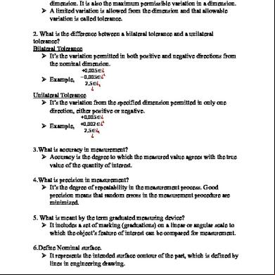
Tutorial 4z844
October 2021 0
Tutorial 4z844
November 2019 114
Tutorial 4z844
September 2022 0
Tutorial 4z844
July 2021 0
Tutorial 4z844
October 2022 0
Tutorial 4z844
December 2022 0More Documents from "Kaustav Patnaik" 4o53m
Tutorial 4z844
October 2022 0
Grit Removal Mechanism 1h5s6i
December 2019 33
Uipath 2a5v1
February 2021 0
Presentation On Price-level ing o4b5y
April 2022 0
Outreach Networks 2m503t
December 2019 54