Arma Arima 50621w

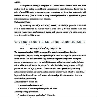
TIME SERIES MODELS – ARMA / ARIMA ARMA Autoregressive Moving-Average (ARMA) models form a class of linear time series models which are widely applicable and parsimonious in parameterization. By allowing the order of an ARMA model to increase, one can approximate any linear time series model with desirable accuracy. [This is similar to using rational polynomials to approximate a general polynomial; see the impulse response function.] Mathematical Model By combining the AR(p) and MA(q) models, an ARMA(p, q) model is obtained. Such a model states that the current value of some series y depends linearly on its own previous values plus a combination of current and previous values of a white noise error term. The model could be written

With

2

E(Ut)=0; E(Ut )= σ2 ; E(Ut Us) = 0, t ≠ s

The characteristics of an ARMA process will be a combination of those from the autoregressive (AR) and moving average (MA) parts. Note that the pacf is particularly useful in this context. The acf alone can distinguish between a pure autoregressive and a pure moving average process. However, an ARMA process will have a geometrically declining acf, as will a pure AR process. So, the pacf is useful for distinguishing between an AR(p) process and an ARMA(p, q) process -- the former will have a geometrically declining autocorrelation function, but a partial autocorrelation function which cuts off to zero after p lags, while the latter will have both autocorrelation and partial autocorrelation functions which decline geometrically. An autoregressive process has:  a geometrically decaying acf  a number of non-zero points of pacf = AR order. A moving average process has:  number of non-zero points of acf = MA order  a geometrically decaying pacf.

A combination autoregressive moving average process has:  a geometrically decaying acf  a geometrically decaying pacf. The autocorrelation function will display combinations of behaviour derived from the AR and MA parts, but for lags beyond q, the acf will simply be identical to the individual AR(p) model, so that the AR part will dominate in the long term. the autoregressive model includes lagged on the time series itself, and that the moving average model includes lagged on the noise or residuals. By including both types of lagged , we arrive at what are called autoregressive-moving-average, or ARMA, models. The order of the ARMA model is included in parentheses as ARMA (p,q), where is the autoregressive order and q the moving-average order. The simplest, and most frequently used ARMA model is ARMA (1,1) model ARIMA ARIMA econometric modeling takes into historical data and decomposes it into an Autoregressive(AR) process where there is a memory of past events (e.g., the interest rate this month is relate to the interest rate last month an so forth with a decreasing memory lag); an Integrated (I) process which s for stabilizing or making the data stationary and ergodic, making it easier ti forecast: and a Moving Average(MA) of the forecast errors , such that the longer the historical data , more accurate the forecasts will be , as it learns over time. ARIMA models therefore have three model parameters, one of the AR(p) process , one of the I(d) process, and one of the MA(q) process all combined and interacting among each other and recomposed in to the ARIMA(p,d,q) model Although the existence of ARMA models predates them, Box and Jenkins (1976) were the first to approach the task of estimating an ARMA model in a systematic manner. Their approach was a practical and pragmatic one, involving these steps  Identification  Estimation  Diagnostic checking

STEPS INVOLVED IN ARMA MODEL  Data should be stationary(it exhibits no trend)  Data should not be non-stationary(it exhibits trend)



If the data is in non-stationary form perform the unit root test and take first difference. Equation for differencing New variable = d (old variable) By then also data is not stationary we have to go for 2nd difference New variable = d (d (old variable))



If the data gets validated then perform correleogram test. Here auto correlation function (MA) and partial auto correlation function (AR) are performed and graphs are plotted.



Equation is estimated in this step with the dependent variable i.e, Depvariable c ar(1) ma(1)



ARMA structure is to be drawn in this the ar values should be inside the circle



Forecasting the values that is shown by graph



Converting in to actual the values that are take are from the differencing then they should be converted to normal by following equations

∆yt = yt – yt-1 Yt = ∆yt+yt-1



By the above process forecasting values of the present data are generated.

Example: Sales forecasting by the given data  Open EVIEWS software and create a WORK FILE, in this example WORKFILE name is SALES  Click FILE option, appears at the leftmost top of the EVIEWS window.  Then a separate window will open then select for UNSTRUCTURED DATA and give NUMBER OF SAMPLES and also give WORKFILE NAME which is OPTIONAL.  Separate WORKFILE window will be opened.  Now copy the SALES data from EXCEL file and paste it on the WORK FILE window, then a new data file is created in the WORKFILE window with the name SERIES 01. Rename the data file for our convenience. Here it is renamed as SALES. 12

6.521942 37.63043 33.23743 15.89615 20.49399 27.99262

19.4698

19.60794 37.74635 49.61371 15.08012 14.34077 37.62316

38.42842 38.87312 40.53457 46.14333

23

18.23048 21.68092

38.37056

33

31.71

23

44.79458 21.01321 34.15229

26

31

42.81324

34

30.77759 9.413606

39.91379

32

42.23344 48.35918 39.52332

6.57869

32.83096 37.02567 46.99541 40.75805 31.12535 16.68686 22 33.78847

26.10266 44.91376 35.65283 37.86205 22.46169 15

47.46016 27.69693 36.17066 22.05206

24 30.00875 28.1 28.333 27.222

27.44772 20.22491 40.85354 19.78139 34.14664

6.40894

28.3211

17.57329 21.88514 33.86894 36.45305

23.5616

18.38318

27.0099

12

12.72301

13.83346 24.13549

22.949

20.19118

31.58513 29.61978 18.87563 17.39709 10.21106 6.839825 25

37.34173

2.16742

40.95237 33.29213 3.418102

25.30864 4.808347 17.98744 22.8835

5.295179 16.15818

38.28979 21.09683 20.96106 10.95136 22.77915 18.85519

26.82028 25.15589 30.24594 10.13787 27.63931 45.36714 20.39776 35.34449 19.1805

33.2634

9.144475

13.2416

34

32.66998 43.13959 2.332049 10.05615

12

17.18094 44.58628 42.18362 0.481683 16.47868 36.00153 24.24151

33

47.88642 0.602427 19.37673 34.65725

15.41568 46.00375 47.38926 14.99983 26.89506 36.36879 12

48.17605 45.13502 22.46767 13.01143

8.827282

22

41.67747 22.89551

5.68487

42.2698 36.21538

UNIT ROOT TEST:  Now open the SALES DATA FILE.  Go to VIEW and click UNIT ROOT TEST.  This test is done to test the stationarity of the data. i.e just to find out whether the data has any upward are downward trend pattern. Null Hypothesis: SALES has a unit root Exogenous: Constant Lag Length: 0 (Automatic - based on SIC, maxlag=13) t-Statistic

Prob.*

Augmented Dickey-Fuller test statistic

-5.433709

0.0000

Test critical values:

1% level

-3.473096

5% level

-2.880211

10% level

-2.576805

*MacKinnon (1996) one-sided p-values.

Augmented Dickey-Fuller Test Equation Dependent Variable: D(SALES)

Method: Least Squares Date: 02/17/12 Time: 00:06 Sample (adjusted): 2 155 Included observations: 154 after adjustments Variable

Coefficient

SALES(-1)

-0.320716

C

Std. Error

t-Statistic

Prob.

0.059023 -5.433709

0.0000

8.569607

1.718684

0.0000

R-squared

0.162651

Mean dependent var

0.097467

Adjusted R-squared

0.157142

S.D. dependent var

9.773778

S.E. of regression

8.973042

Akaike info criterion

7.239229

Sum squared resid

12238.35

Schwarz criterion

7.278670

Log likelihood

-555.4206

F-statistic

29.52519

Prob(F-statistic)

0.000000

4.986144

Hannan-Quinn criter. 7.255249 Durbin-Watson stat

2.057186

   If we observe the above output the probability value is 0.0000, is less than the 0.05, which shows that the data is significantly is stationary. CORRELOGRAM:  Open the same SALES DATA FILE.  Go to VIEW and click CORRELOGRAM.  This test is done to find the Auto Correlation and Partial Correlation values.  The values should be within the dotted lines after few observations

ESTIMATE EQUATION:  Now go to QUICK tab in EVIEWS.  Go to ESTIMATE EQUATION and give the command  Syntax is DEPDNTVARIBLE C AR(1)  In this Equation SALES C AR(1)  Output of this equation is as follows

Dependent Variable: SALES Method: Least Squares Date: 02/17/12 Time: 00:56 Sample (adjusted): 2 155 Included observations: 154 after adjustments Convergence achieved after 3 iterations Variable

Coefficient

Std. Error

t-Statistic

Prob.

C

26.72020

2.255234

11.84808

0.0000

AR(1)

0.679284

0.059023

11.50870

0.0000

R-squared

0.465636

Mean dependent var

26.51376

Adjusted R-squared

0.462120

S.D. dependent var

12.23481

S.E. of regression

8.973042

Akaike info criterion

7.239229

Sum squared resid

12238.35

Schwarz criterion

7.278670

Log likelihood

-555.4206

F-statistic

132.4501

Prob(F-statistic)

0.000000

Inverted AR Roots

Hannan-Quinn criter. 7.255249 Durbin-Watson stat

2.057186

.68

 From the above generated values we say that Auto regression value is below 0.05 from this we say the value is significant.

ARMA STRUCTURE:  In EQUATION dialog box go to VIEW.  Click ARMA Structure.  The AR values generated should be inside the circle.  This is followed if the same process get extended.

FORECAST GRAPH:  In EQUATION dialog box go to FORECAST tab.  From this graph is generated shows FORECASTED values. 60

Forecast: SALESF Actual: SALES Forecast sample: 1 170 Adjusted sample: 2 170 Included observations: 154 Root Mean Squared Error Mean Absolute Error Mean Abs. Percent Error Theil Inequality Coefficient Bias Proportion Variance Proportion Covariance Proportion

50 40 30 20 10 0 -10 25

50

75 SALESF

100

125

± 2 S.E.

 By the above graph values of sales is forecasted.

150

12.29468 10.34978 134.9948 0.220637 0.000000 0.817437 0.182563

CONVERTING INTO ACTUAL 

The values that are generated to be converted and predict in actual values because we consider 1st difference or 2nd difference. Here in this example there is no need as we considered actual values i.e stationary.

FORECASTING USING ARMA MODEL IN EVIEWS EVIEWS provides another piece of useful information -- a decomposition of the forecast errors. The mean squared forecast error can be decomposed into a bias proportion, a variance proportion and a covariance proportion. The bias component measures the extent to which the mean of the forecasts is different to the mean of the actual data (i.e. whether the forecasts are biased). Similarly, the variance component measures the difference between the variation of the forecasts and the variation of the actual data, while the covariance component captures any remaining unsystematic part of the forecast errors.